This page provides a brief overview of MFEM's example codes and miniapps. For
detailed documentation of the MFEM sources, including the examples, see the
online Doxygen documentation,
or the doc directory in the distribution.
The goal of the example codes is to provide a step-by-step introduction to MFEM
in simple model settings. The miniapps are more complex, and are intended to be
more representative of the advanced usage of the library in physics/application
codes. We recommend that new users start with the example codes before moving to
the miniapps.
Select from the categories below to display examples and miniapps that contain the
respective feature. All examples support (arbitrarily) high-order meshes and
finite element spaces.
The numerical results from the example codes can be visualized using the
GLVis visualization tool (based on MFEM). See the
GLVis website for more details.
Users are encouraged to submit any example codes and miniapps that they have created and
would like to share. Contact a member of the MFEM team to report
bugs
or post questions or comments.
Application (PDE)
Finite Elements
Discretization
Solver
Example 0: Simplest Poisson Problem
This is the simplest MFEM example and a good starting point for new users.
The example demonstrates the use of MFEM to define and solve an $H^1$ finite
element discretization of the Poisson equation
$$-\Delta u = 1 \quad\text{in } \Omega$$
with homogeneous Dirichlet boundary conditions
$$ u = 0 \quad\text{on } \partial\Omega$$
The example illustrates the use of the basic MFEM classes for defining the mesh,
finite element space, as well as linear and bilinear forms corresponding to the
left-hand side and right-hand side of the discrete linear system.
The example has serial (ex0.cpp)
and parallel (ex0p.cpp)
versions.
Example 1: Poisson Problem
This example code demonstrates the use of MFEM to define a simple isoparametric
finite element discretization of the Poisson equation $$-\Delta u = 1$$ with
homogeneous Dirichlet boundary conditions. Specifically, we discretize with the
finite element space coming from the mesh (linear by default, quadratic for
quadratic curvilinear mesh, NURBS for NURBS mesh, etc.) The problem solved in
this example is the same as ex0, but with more sophisticated options and
features.
The example highlights the use of mesh refinement, finite element grid
functions, as well as linear and bilinear forms corresponding to the left-hand
side and right-hand side of the discrete linear system. We also cover the
explicit elimination of essential boundary conditions, static condensation, and
the optional connection to the GLVis tool for visualization.
This example code solves a simple linear elasticity problem
describing a multi-material cantilever beam.
Specifically, we approximate the weak form of
$$-{\rm div}({\sigma}({\bf u})) = 0$$
where
$${\sigma}({\bf u}) = \lambda\, {\rm div}({\bf u})\,I + \mu\,(\nabla{\bf u} + \nabla{\bf u}^T)$$
is the stress tensor corresponding to displacement field ${\bf u}$, and $\lambda$ and $\mu$
are the material Lame constants. The boundary conditions are
${\bf u}=0$ on the fixed part of the boundary with attribute 1, and
${\sigma}({\bf u})\cdot n = f$ on the remainder with $f$ being
a constant pull down vector on boundary elements with attribute 2, and zero
otherwise. The geometry of the domain is assumed to be as follows:
The example demonstrates the use of high-order and NURBS vector
finite element spaces with the linear elasticity bilinear form,
meshes with curved elements, and the definition of piece-wise
constant and vector coefficient objects. Static condensation is
also illustrated.
The example has a serial (ex2.cpp)
and a parallel (ex2p.cpp) version.
It also has a PETSc modification in examples/petsc
and a PUMI modification in examples/pumi.
We recommend viewing Example 1 before viewing this example.
Example 3: Definite Maxwell Problem
This example code solves a simple 3D electromagnetic diffusion
problem corresponding to the second order definite Maxwell
equation $$\nabla\times\nabla\times\, E + E = f$$
with boundary condition $ E \times n $ = "given tangential field".
Here, we use a given exact solution $E$ and compute the corresponding r.h.s.
$f$. We discretize with Nedelec finite elements in 2D or 3D.
The example demonstrates the use of $H(curl)$ finite element
spaces with the curl-curl and the (vector finite element) mass
bilinear form, as well as the computation of discretization
error when the exact solution is known. Static condensation is
also illustrated.
The example has a serial (ex3.cpp)
and a parallel (ex3p.cpp) version.
It also has a PETSc modification in examples/petsc.
Partial assembly and GPU devices are supported.
We recommend viewing examples 1-2 before viewing this example.
Example 4: Grad-div Problem
This example code solves a simple 2D/3D $H(div)$
diffusion problem corresponding to the second order definite equation
$$-{\rm grad}(\alpha\,{\rm div}(F)) + \beta F = f$$
with boundary condition $F \cdot n$ = "given normal field".
Here we use a given exact solution $F$ and compute the corresponding
right hand side $f$. We discretize with the Raviart-Thomas finite elements.
The example demonstrates the use of $H(div)$
finite element spaces with the grad-div and $H(div)$
vector finite element mass bilinear form, as well as the computation of discretization
error when the exact solution is known.
Bilinear form hybridization and static condensation are also illustrated.
The example has a serial (ex4.cpp)
and a parallel (ex4p.cpp) version.
It also has a PETSc modification in examples/petsc.
Partial assembly and GPU devices are supported.
We recommend viewing examples 1-3 before viewing this example.
Example 5: Darcy Problem
This example code solves a simple 2D/3D mixed Darcy problem
corresponding to the saddle point system
$$ \begin{array}{rcl}
k\,{\bf u} + {\rm grad}\,p &=& f \\
-{\rm div}\,{\bf u} &=& g
\end{array} $$
with natural boundary condition $-p = $ "given pressure".
Here we use a given exact solution $({\bf u},p)$ and compute the
corresponding right hand side $(f, g)$. We discretize with Raviart-Thomas
finite elements (velocity $\bf u$) and piecewise discontinuous
polynomials (pressure $p$).
The example demonstrates the use of the BlockMatrix and BlockOperator
classes, as well as the collective saving of several grid functions in
VisIt and ParaView
formats.
The example has a serial (ex5.cpp)
and a parallel (ex5p.cpp) version.
It also has a PETSc modification in examples/petsc.
Partial assembly is supported.
We recommend viewing examples 1-4 before viewing this example.
Example 6: Poisson Problem with AMR
This is a version of Example 1 with a simple adaptive mesh
refinement loop. The problem being solved is again the Poisson
equation $$-\Delta u = 1$$ with homogeneous Dirichlet boundary
conditions. The problem is solved on a sequence of meshes which
are locally refined in a conforming (triangles, tetrahedrons)
or non-conforming (quadrilaterals, hexahedra) manner according
to a simple ZZ error estimator.
The example demonstrates MFEM's capability to work with both
conforming and nonconforming refinements, in 2D and 3D, on
linear, curved and surface meshes. Interpolation of functions
from coarse to fine meshes, as well as persistent GLVis
visualization are also illustrated.
The example has a serial (ex6.cpp)
and a parallel (ex6p.cpp) version.
It also has a PETSc modification in examples/petsc
and a PUMI modification in examples/pumi.
Partial assembly and GPU devices are supported.
We recommend viewing Example 1 before viewing this example.
Example 7: Surface Meshes
This example code demonstrates the use of MFEM to define a
triangulation of a unit sphere and a simple isoparametric
finite element discretization of the screened Poisson equation,
$$-\Delta u + u = f.$$
The example highlights mesh generation, the use of mesh
refinement, high-order meshes and finite elements, as well as
surface-based linear and bilinear forms corresponding to the
left-hand side and right-hand side of the discrete linear
system. Simple local mesh refinement is also demonstrated.
The example has a serial (ex7.cpp)
and a parallel (ex7p.cpp) version.
We recommend viewing Example 1 before viewing this example.
Example 8: DPG for the Poisson Problem
This example code demonstrates the use of the Discontinuous
Petrov-Galerkin (DPG) method in its primal 2x2 block form as a
simple finite element discretization of the Poisson problem
$$-\Delta u = f$$ with homogeneous Dirichlet boundary conditions. We
use high-order continuous trial space, a high-order interfacial
(trace) space, and a high-order discontinuous test space
defining a local dual ($H^{-1}$) norm.
We use the primal form of DPG, see
"A primal DPG method without a first-order reformulation",
Demkowicz and Gopalakrishnan, CAM 2013.
The example highlights the use of interfacial (trace) finite
elements and spaces, trace face integrators and the definition
of block operators and preconditioners.
The example has a serial (ex8.cpp)
and a parallel (ex8p.cpp) version.
We recommend viewing examples 1-5 before viewing this example.
Example 9: DG Advection
This example code solves the time-dependent advection equation
$$\frac{\partial u}{\partial t} + v \cdot \nabla u = 0,$$ where $v$ is a given fluid
velocity, and $u_0(x)=u(0,x)$ is a given initial condition.
The example demonstrates the use of Discontinuous Galerkin (DG) bilinear forms
in MFEM (face integrators), the use of explicit and implicit (with block ILU
preconditioning) ODE time integrators, the definition of periodic boundary
conditions through periodic meshes, as well as the use of
GLVis for persistent visualization of a time-evolving
solution. The saving of time-dependent data files for external visualization
with VisIt and ParaView is also illustrated.
This example solves a time dependent nonlinear elasticity problem of the form
$$ \frac{dv}{dt} = H(x) + S v\,,\qquad \frac{dx}{dt} = v\,, $$
where $H$ is a hyperelastic model and $S$ is a viscosity operator of
Laplacian type. The geometry of the domain is assumed to be as follows:
The example demonstrates the use of nonlinear operators, as well as their
implicit time integration using a Newton method for solving an associated
reduced backward-Euler type nonlinear equation. Each Newton step requires the
inversion of a Jacobian matrix, which is done through a (preconditioned) inner
solver.
The example has a serial (ex10.cpp)
and a parallel (ex10p.cpp) version.
It also has a SUNDIALS modification in examples/sundials
and a PETSc modification in examples/petsc.
We recommend viewing examples 2 and 9 before viewing this example.
Example 11: Laplacian Eigenproblem
This example code demonstrates the use of MFEM to solve the eigenvalue problem
$$-\Delta u = \lambda u$$ with homogeneous Dirichlet boundary conditions.
We compute a number of the lowest eigenmodes by discretizing the Laplacian and
Mass operators using a finite element space of the specified order, or an
isoparametric/isogeometric space if order < 1 (quadratic for quadratic
curvilinear mesh, NURBS for NURBS mesh, etc.)
The example highlights the use of the LOBPCG eigenvalue solver together with the
BoomerAMG preconditioner in HYPRE, as well as optionally the SuperLU or
STRUMPACK parallel direct solvers. Reusing a single GLVis
visualization window for multiple eigenfunctions is also illustrated.
The example has only a parallel
(ex11p.cpp) version.
It also has a SLEPc modification in examples/petsc.
We recommend viewing Example 1 before viewing this example.
Example 12: Linear Elasticity Eigenproblem
This example code solves the linear elasticity eigenvalue
problem for a multi-material cantilever beam.
Specifically, we compute a number of the lowest eigenmodes by approximating the weak form of
$$-{\rm div}({\sigma}({\bf u})) = \lambda {\bf u} \,,$$
where
$${\sigma}({\bf u}) = \lambda\, {\rm div}({\bf u})\,I + \mu\,(\nabla{\bf u} + \nabla{\bf u}^T)$$
is the stress tensor corresponding to displacement field $\bf u$, and $\lambda$ and $\mu$
are the material Lame constants. The boundary conditions are
${\bf u}=0$ on the fixed part of the boundary with attribute 1, and
${\sigma}({\bf u})\cdot n = f$ on the remainder.
The geometry of the domain is assumed to be as follows:
The example highlights the use of the LOBPCG eigenvalue solver together with the
BoomerAMG preconditioner in HYPRE.
Reusing a single GLVis visualization window for multiple
eigenfunctions is also illustrated.
The example has only a parallel
(ex12p.cpp) version.
We recommend viewing examples 2 and 11 before viewing this example.
Example 13: Maxwell Eigenproblem
This example code solves the Maxwell (electromagnetic)
eigenvalue problem
$$\nabla\times\nabla\times\, E = \lambda\, E $$
with homogeneous Dirichlet boundary conditions $E \times n = 0$.
We compute a number of the lowest nonzero eigenmodes by
discretizing the curl curl operator using a Nedelec finite element space of
the specified order in 2D or 3D.
The example highlights the use of the AME subspace eigenvalue
solver from HYPRE, which uses LOBPCG and AMS internally.
Reusing a single GLVis visualization window for multiple
eigenfunctions is also illustrated.
The example has only a parallel
(ex13p.cpp) version.
We recommend viewing examples 3 and 11 before viewing this example.
Example 14: DG Diffusion
This example code demonstrates the use of MFEM to define a
discontinuous Galerkin (DG) finite element discretization of
the Poisson equation $$-\Delta u = 1$$ with homogeneous Dirichlet
boundary conditions. Finite element spaces of any order,
including zero on regular grids, are supported. The example highlights the use
of discontinuous spaces and DG-specific face integrators.
The example has a serial (ex14.cpp)
and a parallel (ex14p.cpp) version.
We recommend viewing examples 1 and 9 before viewing this example.
Example 15: Dynamic AMR
Building on Example 6, this example demonstrates dynamic adaptive mesh refinement.
The mesh is adapted to a time-dependent solution by refinement
as well as by derefinement. For simplicity, the solution is
prescribed and no time integration is done. However, the error
estimation and refinement/derefinement decisions are realistic.
At each outer iteration the right hand side function is changed
to mimic a time dependent problem. Within each inner iteration
the problem is solved on a sequence of meshes which are locally
refined according to a simple ZZ error estimator. At the end
of the inner iteration the error estimates are also used to
identify any elements which may be over-refined and a single
derefinement step is performed. After each refinement or
derefinement step a rebalance operation is performed to keep
the mesh evenly distributed among the available processors.
The example demonstrates MFEM's capability to refine, derefine
and load balance nonconforming meshes, in 2D and 3D, and on
linear, curved and surface meshes. Interpolation of functions
between coarse and fine meshes, persistent GLVis visualization,
and saving of time-dependent fields for external visualization
with VisIt are also illustrated.
The example has a serial (ex15.cpp)
and a parallel (ex15p.cpp) version.
We recommend viewing examples 1, 6 and 9 before viewing this example.
Example 16: Time Dependent Heat Conduction
This example code solves a simple 2D/3D time dependent nonlinear heat conduction problem
$$\frac{du}{dt} = \nabla \cdot \left( \kappa + \alpha u \right) \nabla u$$
with a natural insulating boundary condition $\frac{du}{dn} = 0$.
We linearize the problem by using the temperature field $u$ from the previous time
step to compute the conductivity coefficient.
This example demonstrates both implicit and explicit time integration as well as a single
Picard step method for linearization. The saving of time dependent data files for external
visualization with VisIt is also illustrated.
The example has a serial (ex16.cpp)
and a parallel (ex16p.cpp) version.
We recommend viewing examples 2, 9, and 10 before viewing this example.
Example 17: DG Linear Elasticity
This example code solves a simple linear elasticity problem
describing a multi-material cantilever beam using symmetric or
non-symmetric discontinuous Galerkin (DG) formulation.
Specifically, we approximate the weak form of
$$-{\rm div}({\sigma}({\bf u})) = 0$$
where
$${\sigma}({\bf u}) = \lambda\, {\rm div}({\bf u})\,I + \mu\,(\nabla{\bf u} + \nabla{\bf u}^T)$$
is the stress tensor corresponding to displacement field ${\bf u}$, and $\lambda$ and $\mu$
are the material Lame constants. The boundary conditions are
Dirichlet, $\bf{u}=\bf{u_D}$, on the fixed part of the boundary, namely
boundary attributes 1 and 2; on the rest of the boundary we use
${\sigma}({\bf u})\cdot n = {\bf 0}$. The geometry of the domain is assumed to be
as follows:
The example demonstrates the use of high-order DG vector finite
element spaces with the linear DG elasticity bilinear form,
meshes with curved elements, and the definition of piece-wise
constant and function vector-coefficient objects. The use of
non-homogeneous Dirichlet b.c. imposed weakly, is also
illustrated.
The example has a serial (ex17.cpp)
and a parallel (ex17p.cpp) version.
We recommend viewing examples 2 and 14 before viewing this example.
Example 18: DG Euler Equations
This example code solves the compressible Euler system of equations, a model
nonlinear hyperbolic PDE, with a discontinuous Galerkin (DG) formulation. The
primary purpose is to show how a transient system of nonlinear equations can be
formulated in MFEM. The equations are solved in conservative form
with a state vector $u = [ \rho, \rho v_0, \rho v_1, \rho E ]$, where $\rho$ is
the density, $v_i$ is the velocity in the $i^{\rm th}$ direction, $E$ is the
total specific energy, and $H = E + p / \rho$ is the total specific enthalpy.
The pressure, $p$ is computed through a simple equation of state (EOS) call.
The conservative hydrodynamic flux ${\bf F}$ in each direction $i$ is
$${\bf F_{\it i}} = [ \rho v_i, \rho v_0 v_i + p \delta_{i,0}, \rho v_1 v_i + p \delta_{i,1}, \rho v_i H ]$$
Specifically, the example solves for an exact solution of the equations whereby
a vortex is transported by a uniform flow. Since all boundaries are periodic
here, the method's accuracy can be assessed by measuring the difference between
the solution and the initial condition at a later time when the vortex returns
to its initial location.
Note that as the order of the spatial discretization increases, the timestep
must become smaller. This example currently uses a simple estimate derived by
Cockburn and Shu
for the 1D RKDG method. An additional factor can be tuned by passing the --cfl
(or -c shorter) flag.
The example demonstrates user-defined nonlinear form with hyperbolic form
integrator for systems of equations that are defined with block vectors,
and how these are used with an operator for explicit time integrators.
In this case the system also involves an external approximate Riemann
solver for the DG interface flux. It also demonstrates how to use GLVis
for in-situ visualization of vector grid functions.
The example has a serial (ex18.cpp)
and a parallel (ex18p.cpp) version.
We recommend viewing examples 9, 14 and 17 before viewing this example.
Example 19: Incompressible Nonlinear Elasticity
This example code solves the quasi-static incompressible nonlinear
hyperelasticity equations. Specifically, it solves the nonlinear equation
$$
\nabla \cdot \sigma(F) = 0
$$
subject to the constraint
$$
\text{det } F = 1
$$
where $\sigma$ is the Cauchy stress and $F_{ij} = \delta_{ij} + u_{i,j}$ is the deformation
gradient. To handle the incompressibility constraint, pressure is included as
an independent unknown $p$ and the stress response is modeled as an incompressible
neo-Hookean hyperelastic solid.
The geometry of the domain is assumed to be as follows:
This formulation requires solving the saddle point system
$$ \left[ \begin{array}{cc}
K &B^T \\
B & 0
\end{array} \right]
\left[\begin{array}{c} \Delta u \\ \Delta p \end{array} \right] =
\left[\begin{array}{c} R_u \\ R_p \end{array} \right]
$$
at each Newton step. To solve this linear system, we implement a specialized block
preconditioner of the form
$$
P^{-1} =
\left[\begin{array}{cc} I & -\tilde{K}^{-1}B^T \\ 0 & I \end{array} \right]
\left[\begin{array}{cc} \tilde{K}^{-1} & 0 \\ 0 & -\gamma \tilde{S}^{-1} \end{array} \right]
$$
where $\tilde{K}^{-1}$ is an approximation of the inverse of the stiffness matrix $K$ and
$\tilde{S}^{-1}$ is an approximation of the inverse of the Schur complement $S = BK^{-1}B^T$.
To approximate the Schur complement, we use the mass matrix for the pressure variable $p$.
The example demonstrates how to solve nonlinear systems of equations that are defined with
block vectors as well as how to implement specialized block preconditioners for use in
iterative solvers.
The example has a serial (ex19.cpp)
and a parallel (ex19p.cpp) version.
We recommend viewing examples 2, 5 and 10 before viewing this example.
Example 20: Symplectic Integration of Hamiltonian Systems
This example demonstrates the use of the variable order, symplectic time
integration algorithm. Symplectic integration algorithms are designed to
conserve energy when integrating systems of ODEs which are derived from
Hamiltonian systems.
Hamiltonian systems define the energy of a system as a function of
time (t), a set of generalized coordinates (q), and their corresponding
generalized momenta (p).
$$
H(q,p,t) = T(p) + V(q,t)
$$
Hamilton's equations then specify how q and p evolve in time:
$$
\frac{dq}{dt} = \frac{dH}{dp}\,,\qquad
\frac{dp}{dt} = -\frac{dH}{dq}
$$
To use the symplectic integration classes we need to define an mfem::Operator
${\bf P}$ which evaluates the action of dH/dp, and an
mfem::TimeDependentOperator ${\bf F}$ which computes -dH/dq.
This example visualizes its results as an evolution in phase space by defining
the axes to be $q$, $p$, and $t$ rather than $x$, $y$, and $z$. In this space
we build a ribbon-like mesh with nodes at $(0,0,t)$ and $(q,p,t)$. Finally we
plot the energy as a function of time as a scalar field on this ribbon-like
mesh. This scheme highlights any variations in the energy of the system.
This example offers five simple 1D Hamiltonians:
Simple Harmonic Oscillator (mass on a spring)
$$H = \frac{1}{2}\left( \frac{p^2}{m} + \frac{q^2}{k} \right)$$
In all cases these Hamiltonians are shifted by constant values so that the
energy will remain positive. The mean and standard deviation of the computed
energies at each time step are displayed upon completion.
When run in parallel, each processor integrates the same Hamiltonian
system but starting from different initial conditions.
The example has a serial (ex20.cpp)
and a parallel (ex20p.cpp) version.
See the Maxwell miniapp for another
application of symplectic integration.
Example 21: Adaptive mesh refinement for linear elasticity
This is a version of Example 2 with a simple adaptive mesh
refinement loop. The problem being solved is again linear
elasticity describing a multi-material cantilever beam.
The problem is solved on a sequence of meshes which
are locally refined in a conforming (triangles, tetrahedrons)
or non-conforming (quadrilaterals, hexahedra) manner according
to a simple ZZ error estimator.
The example demonstrates MFEM's capability to work with both
conforming and nonconforming refinements, in 2D and 3D, on
linear and curved meshes. Interpolation of functions from
coarse to fine meshes, as well as persistent GLVis
visualization are also illustrated.
The example has a serial (ex21.cpp)
and a parallel (ex21p.cpp) version.
We recommend viewing Examples 2 and 6 before viewing this example.
Example 22: Complex Linear Systems
This example code demonstrates the use of MFEM to define and
solve a complex-valued linear system. It implements three variants
of a damped harmonic oscillator:
In each case the field is driven by a forced oscillation, with
angular frequency $\omega$, imposed at the boundary or a portion
of the boundary.
The example also demonstrates how to display a time-varying solution as
a sequence of fields sent to a single GLVis socket.
The example has a serial (ex22.cpp)
and a parallel (ex22p.cpp) version.
We recommend viewing examples 1, 3, and 4 before viewing this example.
Example 23: Wave Problem
This example code solves a simple 2D/3D wave
equation with a second order time derivative:
$$\frac{\partial^2 u}{\partial t^2} - c^2\Delta u = 0$$
The boundary conditions are either Dirichlet or Neumann.
The example demonstrates the use of time dependent operators,
implicit solvers and second order time integration.
The example has only a serial (ex23.cpp) version.
We recommend viewing examples 9 and 10 before viewing this example.
Example 24: Mixed finite element spaces
This example code illustrates usage of mixed finite element
spaces, with three variants:
$H^1 \times H(curl)$
$H(curl) \times H(div)$
$H(div) \times L_2$
Using different approaches for demonstration purposes, we project or interpolate a gradient, curl, or
divergence in the appropriate spaces, comparing the errors in each case.
The example has a serial (ex24.cpp)
and a parallel (ex24p.cpp) version.
We recommend viewing examples 1 and 3 before viewing this example.
Example 25: Perfectly Matched Layers
The example illustrates the use of a Perfectly Matched Layer (PML) for the
simulation of time-harmonic electromagnetic waves propagating in unbounded
domains.
PML was originally introduced by Berenger in "A Perfectly Matched Layer for the
Absorption of Electromagnetic Waves".
It is a technique used to solve wave propagation problems posed in infinite
domains. The implementation involves the introduction of an artificial absorbing
layer that minimizes undesired reflections. Inside this layer a complex
coordinate stretching map is used which forces the wave modes to decay
exponentially.
The example solves the indefinite Maxwell equations
$$\nabla \times (a \nabla \times E) - \omega^2 b E = f.$$
where $a = \mu^{-1} |J|^{-1} J^T J$, $b= \epsilon |J| J^{-1} J^{-T}$ and $J$ is
the Jacobian matrix of the coordinate transformation.
The example demonstrates discretization with Nedelec finite elements in 2D or
3D, as well as the use of complex-valued bilinear and linear forms. Several
test problems are included, with known exact solutions.
The example has a serial (ex25.cpp)
and a parallel (ex25p.cpp) version.
We recommend viewing Example 22 before viewing this example.
Example 26: Multigrid Preconditioner
This example code demonstrates the use of MFEM to define a
simple isoparametric finite element discretization of the
Poisson equation $$-\Delta u = 1$$ with homogeneous Dirichlet
boundary conditions and how to solve it efficiently using a
matrix-free multigrid preconditioner.
The example highlights on the creation of a hierarchy of
discretization spaces and diffusion bilinear forms using
partial assembly. The levels in the hierarchy of finite
element spaces maybe constructed through geometric or
order refinements. Moreover, the construction of a multigrid
preconditioner for the PCG solver is shown. The multigrid
uses a PCG solver on the coarsest level and second order
Chebyshev accelerated smoothers on the other levels.
The example has a serial (ex26.cpp)
and a parallel (ex26p.cpp) version.
We recommend viewing Example 1 before viewing this example.
Example 27: Boundary Conditions for the Laplace Problem
This example code demonstrates the use of MFEM to define a
simple finite element discretization of Laplace's equation:
$$
-\Delta u = 0
$$
with a variety of boundary conditions.
Specifically, we discretize
using a FE space of the specified order using a continuous or
discontinuous space. We then apply Dirichlet, Neumann (both
homogeneous and inhomogeneous), Robin, and Periodic boundary
conditions on different portions of a predefined mesh.
Boundary conditions:
$u = u_{dbc}$
on $\Gamma_{dbc}$
$\hat{n}\cdot\nabla u = g_{nbc}$
on $\Gamma_{nbc}$
$\hat{n}\cdot\nabla u = 0$
on $\Gamma_{nbc_0}$
$\hat{n}\cdot\nabla u + a u = b$
on $\Gamma_{rbc}$
as well as periodic boundary conditions which are enforced topologically.
The example has a serial (ex27.cpp)
and a parallel (ex27p.cpp) version.
We recommend viewing examples 1 and 14 before viewing this example.
Example 28: Constraints and Sliding Boundary Conditions
This example code illustrates the use of constraints in linear solvers by
solving an elasticity problem where the normal component of the displacement
is constrained to zero on two boundaries but tangential displacement is
allowed.
The constraints can be enforced in several different ways, including
eliminating them from the linear system or solving a saddle-point
system that explicitly includes constraint conditions.
The example has a serial (ex28.cpp)
and a parallel (ex28p.cpp) version.
We recommend viewing example 2 before viewing this example.
Example 29: Solving PDEs on embedded surfaces
This example demonstrates setting up and solving an anisotropic Poisson problem
$$-\nabla\cdot(\sigma\nabla u) = 1 \quad\text{in } \Omega$$
with homogeneous Dirichlet boundary conditions
$$ u = 0 \quad\text{on } \partial\Omega$$
where $\Omega$ is a two dimensional curved surface embedded in three
dimensions and $\sigma$ is an anisotropic diffusion tensor.
The example demonstrates and validates our DiffusionIntegrator's ability to
properly integrate three dimensional fluxes on a two dimensional domain. Not
all of our integrators currently support such cases but the
DiffusionIntegrator can be used as a simple example of how extend other
integrators when necessary.
The example has a serial (ex29.cpp)
and a parallel (ex29p.cpp) version.
We recommend viewing examples 1 and 7 before viewing this example.
Example 30: Resolving rough and fine-scale problem data
Unresolved problem data will affect the accuracy of a discretized PDE solution as
well as a posteriori estimates of the solution error.
This example uses a CoefficientRefiner object to preprocess an input mesh until
the resolution of the prescribed problem data $f \in L^2$ is below a prescribed
tolerance. In this example, the resolution is identified with a data oscillation
function on the mesh $\mathcal{T}$, defined
$$ \mathrm{osc}(f) = \Big( \sum_{T\in\mathcal{T}} \| h \cdot (I - \Pi)\, f \|^2_{L^2(T)} \Big)^{1/2}, $$
where $h$ is the local element size function and $\Pi$ is a finite element projection
operator, and the sum is taken over all elements $T$ in the mesh.
In this example, the coarse initial mesh is adaptively refined until $\mathrm{osc}(f)$ is below a
prescribed tolerance for various candidate functions $f \in L^2$. When using rough problem data,
it is recommended to perform this type of preprocessing before a posteriori error estimation.
The example has a serial (ex30.cpp)
and a parallel (ex30p.cpp) version.
We recommend viewing examples 1 and 6 before viewing this example.
Example 31: Anisotropic Definite Maxwell Problem
This example code solves a simple electromagnetic diffusion
problem corresponding to the second order definite Maxwell
equation $$\nabla\times\nabla\times\, E + \sigma E = f$$
with boundary condition $ E \times n $ = "given tangential field".
In this example $\sigma$ is an anisotropic 3x3 tensor. Here, we use a
given exact solution $E$ and compute the corresponding r.h.s.
$f$. We discretize with Nedelec finite elements in 1D, 2D, or 3D.
The example demonstrates the use of restricted $H(curl)$ finite element
spaces with the curl-curl and the (vector finite element) mass
bilinear form, as well as the computation of discretization
error when the exact solution is known. These restricted spaces allow
the solution of 1D or 2D electromagnetic problems which involve 3D
field vectors. Such problems arise in plasma physics and crystallography.
The example has a serial (ex31.cpp)
and a parallel (ex31p.cpp) version.
We recommend viewing example 3 before viewing this example.
Example 32: Anisotropic Maxwell Eigenproblem
This example code solves the Maxwell (electromagnetic)
eigenvalue problem with anisotropic permittivity, $\epsilon$
$$\nabla\times\nabla\times\, E = \lambda\, \epsilon E $$
with homogeneous Dirichlet boundary conditions $E \times n = 0$.
We compute a number of the lowest nonzero eigenmodes by
discretizing the curl curl operator using a Nedelec finite element space of
the specified order in 1D, 2D, or 3D.
The example demonstrates the use of restricted $H(curl)$ finite element
spaces in an eigenmode context. These restricted spaces allow
the solution of 1D or 2D electromagnetic problems which involve 3D
field vectors. Such problems arise in plasma physics and crystallography.
The example highlights the use of the AME subspace eigenvalue
solver from HYPRE, which uses LOBPCG and AMS internally.
Reusing multiple GLVis visualization windows for multiple
eigenfunctions is also illustrated.
The example has only a parallel
(ex32p.cpp) version.
We recommend viewing examples 13 and 31 before viewing this example.
Example 33: Spectral fractional Laplacian
This example code demonstrates the use of MFEM to solve the fractional Laplacian problem
$$ (-\Delta)^\alpha u = 1, \quad \alpha > 0, $$
with homogeneous Dirichlet boundary conditions. The problem solved in this example is similar to
ex1, but involves a fractional-order diffusion operator whose inverse can be approximated
by a series of inverses of integer-order diffusion operators. Solving each of these independent
integer-order PDEs with MFEM and summing their solutions results in a discrete solution to the
fractional Laplacian problem above.
The example has a serial (ex33.cpp)
and a parallel (ex33p.cpp) version.
We recommend viewing Example 1 before viewing this example.
Example 34: Source Function using a SubMesh Transfer
This example demonstrates the use of a SubMesh object to transfer solution
data from a sub-domain and use this as a source function on the full domain.
In this case we compute a volumetric current density $\vec{J}$ as the gradient
of a scalar potential $\varphi$ on a portion of the domain.
Where a voltage difference is applied on surfaces of the sub-domain (shown on
the left) to generate the current density restricted to this sub-domain. The
current density is then transferred to the full domain (shown on the right)
using a SubMesh object.
We then use this current density on the full domain as a source term in a
magnetostatic solve for a vector potential $\vec{A}$.
This example verifies the recreation of boundary attributes on a sub-domain
mesh as well as transfer of Raviart-Thomas vector fields between the SubMesh
and the full Mesh. Note that the data transfer in this particular example
involves arbitrary order Raviart-Thomas degrees of freedom on a mixture of
tetrahedral and triangular prism elements.
The example has a serial (ex34.cpp)
and a parallel (ex34p.cpp) version.
We recommend viewing Examples 1 and 3 before viewing this example.
Example 35: Port Boundary Conditions using SubMesh Transfers
This example demonstrates the use of a SubMesh object to transfer a port
boundary condition from a portion of the boundary to the corresponding portion
of the full domain.
Just as in Example 22 this example implements three variants of a damped
harmonic oscillator:
A scalar $H^1$ field:
$$-\nabla\cdot\left(a \nabla u\right) - \omega^2 b\,u + i\,\omega\,c\,u = 0\mbox{ with }u|_\Gamma=v$$
A vector $H(curl)$ field:
$$\nabla\times\left(a\nabla\times\vec{u}\right) - \omega^2 b\,\vec{u} + i\,\omega\,c\,\vec{u} = 0\mbox{ with }\hat{n}\times(\vec{u}\times\hat{n})|_\Gamma=\vec{v}$$
A vector $H(div)$ field:
$$-\nabla\left(a \nabla\cdot\vec{u}\right) - \omega^2 b\,\vec{u} + i\,\omega\,c\,\vec{u} = 0\mbox{ with }\hat{n}\cdot\vec{u}|_\Gamma=v$$
Where $\Gamma$ is a portion of the boundary called the port. In each case the
field is driven by a forced oscillation, with angular frequency $\omega$,
imposed at the boundary or a portion of the boundary.
In Example 22 this boundary condition was simply a constant in space. In this
example the boundary condition is an eigenmode of a lower dimensional
eigenvalue problem defined on a portion of the boundary as follows:
For the scalar $H^1$ field:
$$-\nabla\cdot\left(\nabla v\right) = \lambda\,v\mbox{ with }v|_{\partial\Gamma}=0$$
For the vector $H(curl)$ field:
$$\nabla\times\left(\nabla\times\vec{v}\right) = \lambda\,\vec{v}\mbox{ with }\hat{n}_{\partial\Gamma}\times\vec{v}|_{\partial\Gamma}=0$$
For the vector $H(div)$ field:
$$-\nabla\cdot\left(\nabla v\right) = \lambda\,v\mbox{ with }\hat{n}_{\partial\Gamma}\cdot\nabla v|_{\partial\Gamma}=0$$
The different cases implemented in this example can be used to verify the
transfer of an $H^1$ scalar field, the tangential components of an $H(curl)$
vector field, and the normal component of an $H(div)$ vector field (as a scalar
$L^2$ field in this case) between a SubMesh and its parent mesh.
The example has only a parallel (ex35p.cpp)
version because the eigenmode solver used to compute the field on the port is
only implemented in parallel. We recommend viewing Examples 11, 13, and 22
before viewing this example.
Example 36: Obstacle Problem
This example code solves the pointwise bound-constrained energy minimization problem
$$ \text{minimize } \frac{1}{2}\|\nabla u\|^2 \text{ in } H^1_0(\Omega)\, \text{ subject to } u \ge \varphi\,.$$
This is known as the obstacle problem, and it is a classical motivating example in the
study of variational inequalities and free boundary problems. In this example, the obstacle $\varphi$
is the graph of a half-sphere centered at the origin of a circular domain $\Omega$. After solving to
a specified tolerance, the numerical solution is compared to a closed-form exact solution to assess
its accuracy.
The problem is solved using the Proximal Galerkin finite element method, which is a nonlinear,
structure-preserving mixed method for pointwise bound constraints proposed by
Keith and Surowiec. In turn, this example highlights
MFEM's ability to deliver high-order solutions to variational inequalities and showcases how to
set up and solve nonlinear mixed methods.
The example has a serial (ex36.cpp)
and a parallel (ex36p.cpp) version.
We recommend viewing Example 1 before viewing this example.
Example 37: Topology Optimization
Density field $\rho$
Problem set-up and domain $\Omega$
This example code solves a classical cantilever beam topology optimization problem.
The aim is to find an optimal material density field $\rho$ in $L^1(\Omega)$ to minimize the elastic compliance; i.e.,
$$\begin{align}
&\text{minimize} \int_\Omega \mathbf{f} \cdot \mathbf{u}(\rho)\, \mathrm{d}x\,
\text{ over }\, \rho \in L^1(\Omega)
\\
&\text{subject to }\, 0 \leq \rho \leq 1\, \text{ and } \int_\Omega \rho\, \mathrm{d}x = \theta\, \mathrm{vol}(\Omega) \,.
\end{align}$$
In this problem, $\mathbf{f}$ is a localized force and the linearly elastic displacement field $\mathbf{u} = \mathbf{u}(\rho)$ is determined by a material density field $\rho$ with total volume fraction $0<\theta<1$.
The problem is solved using a mirror descent algorithm proposed by Keith and Surowiec.
For further details, see the more elaborate description of this PDE-constrained optimization problem given in the example code and the aforementioned paper.
The example has a serial (ex37.cpp)
and a parallel (ex37p.cpp) version.
We recommend viewing Example 2 before viewing this example.
Example 38: Cut-Volume and Cut-Surface Integration
This example code demonstrates construction of cut-surface and cut-volume IntegrationRules.
The cut is specified by the zero level set of a given Coefficient $\phi$.
The resulting IntegrationRules are combined with standard LinearFormIntegrators to demonstrate
integration of a function $u$ over an implicit interface, and a subdomain bounded by an implicit interface:
$$ S = \int_{\phi = 0} u(x) ~ ds, \quad V = \int_{\phi > 0} u(x) ~ dx. $$
The IntegrationRules are constructed by the moment-fitting algorithm introduced by
Müller, Kummer and Oberlack. Through a set of basis functions,
for each element the method defines and solves a local under-determined system for the vector of quadrature weights.
All surface and volume integrals, which are required to form the system, are reduced to 1D integration over intersected segments.
The example has only a serial (ex38.cpp)
version, because the construction of the integration rules is an element-local procedure.
It requires MFEM to be built with LAPACK, which is used to find the optimal solution of an under-determined system of equations.
Example 39: Named Attribute Sets
This example uses the Poisson equation to demonstrate the use of named attribute sets in MFEM to specify material regions, boundary regions, or source regions by name rather than attribute numbers.
It also demonstrates how new named attribute sets may be created from arbitrary groupings of attribute numbers and used as a convenient shorthand to refer to those groupings in other portions of the application or through the command line.
Named attribute sets also required changes to MFEM's mesh file formats.
This example makes use of a custom input mesh file (compass.msh) produced using Gmsh which includes named regions and boundaries.
A related mesh file (compass.mesh) illustrates MFEM's representation of the new named attribute sets.
See file formats for details of the augmented mesh file format.
The example has a serial (ex39.cpp)
and a parallel (ex39p.cpp) version.
We recommend viewing Example 1 before viewing this example.
Example 40: Eikonal Equation
This example highlights MFEM's ability to solve a fully-nonlinear, first-order PDE with high-order finite elements.
In particular this example uses the proximal Galerkin method to solve the eikonal equation,
$$ |\nabla u| = 1 \text{ in } \Omega, \quad u = 0 \text{ on } \partial \Omega. $$
At each point $x$ in the domain $\Omega$, the solution of this PDE provides the Euclidean distance to the domain boundary, $u(x) = \min \{ | x - y| : y \in \partial \Omega\}$.
The problem is solved by recasting $u$ as the solution of the nonlinear program
$$ \text{maximize } \int_\Omega u\, \mathrm{d} x\, \text{ in } W^{1,\infty}_0(\Omega)\, \text{ subject to } |\nabla u | \leq 1 \text{ a.e. in } \Omega.$$
A solution is then obtained by discretizing and solving a sequence of nonlinear saddle-point problems.
See the example code for a more detailed description of the method.
The example has a serial (ex40.cpp)
and a parallel (ex40p.cpp) version.
We recommend viewing Example 5 and Example 36 before viewing this example.
NURBS Example 1: Poisson Problem
This example code demonstrates the use of MFEM to define a simple isogeometric NURBS discretization of
the Poisson equation $$-\Delta u = 1$$ with
homogeneous Dirichlet boundary conditions. The problem solved in
this example is the same as Example 1.
This example code solves a simple electromagnetic diffusion
problem corresponding to the second order definite Maxwell
equation $$\nabla\times\nabla\times\, E + E = f$$
with boundary condition $ E \times n $ = "given tangential field".
Here, we use a given exact solution $E$ and compute the corresponding r.h.s.
$f$. We discretize with NURBS-based $H(curl)$elements in 2D or 3D.
The problem solved in this example is the same as Example 3.
The example has only a serial (nurbs_ex1.cpp) version.
NURBS Example 5: Darcy Problem
This example code solves a simple 2D/3D mixed Darcy problem
corresponding to the saddle point system
$$ \begin{array}{rcl}
k\,{\bf u} + {\rm grad}\,p &=& f \\
-{\rm div}\,{\bf u} &=& g
\end{array} $$
with natural boundary condition $-p = $ "given pressure".
Here we use a given exact solution $({\bf u},p)$ and compute the
corresponding right hand side $(f, g)$. We discretize the velocity ($\bf u$) with NURBS-based $H(div)$ elements and
the pressure ($p$) with a compatible NURBS-based $H_1$ elements.
The problem solved in this example is the same as Example 5.
This example code demonstrates the use of MFEM to solve the eigenvalue problem
$$-\Delta u = \lambda u$$ with homogeneous Dirichlet boundary conditions.
We compute a number of the lowest eigenmodes by discretizing the Laplacian and
Mass operators using a finite element space of the specified order, or an
isoparametric/isogeometric space if order < 1 (quadratic for quadratic
curvilinear mesh, NURBS for NURBS mesh, etc.)
The example highlights the use of the LOBPCG eigenvalue solver together with the
BoomerAMG preconditioner in HYPRE, as well as optionally the SuperLU or
STRUMPACK parallel direct solvers. Reusing a single GLVis
visualization window for multiple eigenfunctions is also illustrated.
The problem solved in this example is the same as Example 11.
The problem solved in this example is the same as Example 24, but NURBS-based elements are also supported.
This example code illustrates usage of mixed finite element
spaces, with three variants:
$H^1 \times H(curl)$
$H(curl) \times H(div)$
$H(div) \times L_2$
Using different approaches for demonstration purposes, we project or interpolate a gradient, curl, or
divergence in the appropriate spaces, comparing the errors in each case.
This miniapp solves the equations of transient full-wave electromagnetics.
Its features include:
mixed formulation of the coupled first-order Maxwell equations
$H(\mathrm{curl})$ discretization of the electric field
$H(\mathrm{div})$ discretization of the magnetic flux
energy conserving, variable order, implicit time integration
dielectric materials
diamagnetic and/or paramagnetic materials
conductive materials
volumetric current densities
Sommerfeld absorbing boundary conditions
high order meshes
high order basis functions
advanced visualization
For more details, please see the documentation in the
miniapps/electromagnetics directory.
The miniapp has only a parallel
(maxwell.cpp) version.
We recommend that new users start with the example codes before
moving to the miniapps.
Joule Miniapp: Transient Magnetics and Joule Heating
This miniapp solves the equations of transient low-frequency (a.k.a. eddy current)
electromagnetics, and simultaneously computes transient heat transfer with the heat source given
by the electromagnetic Joule heating.
Its features include:
$H^1$ discretization of the electrostatic potential
$H(\mathrm{curl})$ discretization of the electric field
$H(\mathrm{div})$ discretization of the magnetic field
$H(\mathrm{div})$ discretization of the heat flux
$L^2$ discretization of the temperature
implicit transient time integration
high order meshes
high order basis functions
adaptive mesh refinement
advanced visualization
For more details, please see the documentation in the
miniapps/electromagnetics directory.
The miniapp has only a parallel
(joule.cpp) version.
We recommend that new users start with the example codes before
moving to the miniapps.
Mobius Strip Miniapp
This miniapp generates various Mobius strip-like surface meshes. It is a good
way to generate complex surface meshes.
Manipulating the mesh topology and performing mesh transformation are demonstrated.
The mobius-strip mesh in the data directory was generated with this miniapp.
For more details, please see the documentation in the
miniapps/meshing directory.
The miniapp has only a serial
(mobius-strip.cpp) version.
We recommend that new users start with the example codes before
moving to the miniapps.
Klein Bottle Miniapp
This miniapp generates three types of Klein bottle surfaces. It is similar to
the mobius-strip miniapp.
Manipulating the mesh topology and performing mesh transformation are demonstrated.
The klein-bottle and klein-donut meshes in the data directory were generated with this miniapp.
For more details, please see the documentation in the
miniapps/meshing directory.
The miniapp has only a serial
(klein-bottle.cpp) version.
We recommend that new users start with the example codes before
moving to the miniapps.
Toroid Miniapp
This miniapp generates two types of toroidal volume meshes; one with
triangular cross sections and one with square cross sections. It
works by defining a stack of individual elements and bending them so
that the bottom and top of the stack can be joined to form a torus. It
supports various options including:
The element type: 0 - Wedge, 1 - Hexahedron
The geometric order of the elements
The major and minor radii
The number of elements in the azimuthal direction
The number of nodes to offset by before rejoining the stack
The initial angle of the cross sectional shape
The number of uniform refinement steps to apply
Along with producing some visually interesting meshes, this miniapp
demonstrates how simple 3D meshes can be constructed and transformed
in MFEM. It also produces a family of meshes with simple but
non-trivial topology for testing various features in MFEM.
This miniapp has only a serial
(toroid.cpp) version.
We recommend that new users start with the example codes before
moving to the miniapps.
Twist Miniapp
This miniapp generates simple periodic meshes to demonstrate MFEM's handling
of periodic domains. MFEM's strategy is to use a discontinuous vector field
to define the mesh coordinates on a topologically periodic mesh. It works by
defining a stack of individual elements and stitching together the top and
bottom of the mesh. The stack can also be twisted so that the vertices of the
bottom and top can be joined with any integer offset (for tetrahedral and
wedge meshes only even offsets are supported).
The Twist miniapp supports various options including:
The element type: 4 - Tetrahedron, 6 - Wedge, 8 - Hexahedron
The geometric order of the elements
The dimensions of the initial brick-shaped stack of elements
The number of elements in the z direction
The number of nodes to offset by before rejoining the stack
The number of uniform refinement steps to apply
Along with producing some visually interesting meshes, this miniapp
demonstrates how simple 3D meshes can be constructed and transformed
in MFEM. It also produces a family of meshes with simple but
non-trivial topology for testing various features in MFEM.
This miniapp has only a serial
(twist.cpp) version.
We recommend that new users start with the example codes before
moving to the miniapps.
Extruder Miniapp
This miniapp creates higher dimensional meshes from lower dimensional meshes
by extrusion. Simple coordinate transformations can also be applied if desired.
The initial mesh can be 1D or 2D
1D meshes can be extruded in both the y and z directions
2D meshes can be triangular, quadrilateral, or contain both element types
Meshes with high order geometry are supported
User can specify the number of elements and the distance to extrude
Geometric order of the transformed mesh can be user selected or automatic
This miniapp provides another demonstration of how simple meshes can be
constructed and transformed in MFEM.
This miniapp has only a serial
(extruder.cpp) version.
We recommend that new users start with the example codes before
moving to the miniapps.
Trimmer Miniapp
This miniapp creates a new mesh file from an existing mesh by trimming away
elements with selected attributes. Newly exposed boundary elements will be
assigned new or user specified boundary attributes.
The initial mesh can be 2D or 3D
Meshes with high order geometry are supported
Periodic meshes are supported
NURBS meshes are not supported
This miniapp provides another demonstration of how simple meshes can be
constructed in MFEM.
This miniapp has only a serial
(trimmer.cpp) version.
We recommend that new users start with the example codes before
moving to the miniapps.
Polar-NC Miniapp
This miniapp generates a circular sector mesh that consist of quadrilaterals
and triangles of similar sizes. The 3D version of the mesh is made of prisms
and tetrahedra.
The mesh is non-conforming by design, and can optionally be made curvilinear.
The elements are ordered along a space-filling curve by default, which makes
the mesh ready for parallel non-conforming AMR in MFEM.
The implementation also demonstrates how to initialize a non-conforming mesh
on the fly by marking hanging nodes with Mesh::AddVertexParents.
For more details, please see the documentation in the
miniapps/meshing directory.
The miniapp has only a serial
(polar-nc.cpp) version.
We recommend that new users start with the example codes before
moving to the miniapps.
Shaper Miniapp
This miniapp performs multiple levels of adaptive mesh refinement to resolve the
interfaces between different "materials" in the mesh, as specified by a given
material function.
It can be used as a simple initial mesh generator, for example in the case when
the interface is too complex to describe without local refinement. Both
conforming and non-conforming refinements are supported.
For more details, please see the documentation in the
miniapps/meshing directory.
The miniapp has only a serial
(shaper.cpp) version.
We recommend that new users start with the example codes before
moving to the miniapps.
Mesh Explorer Miniapp
This miniapp is a handy tool to examine, visualize and manipulate a given
mesh. Some of its features are:
visualizing of mesh materials and individual mesh elements
mesh scaling, randomization, and general transformation
manipulation of the mesh curvature
the ability to simulate parallel partitioning
quantitative and visual reports of mesh quality
For more details, please see the documentation in the
miniapps/meshing directory.
The miniapp has only a serial
(mesh-explorer.cpp) version.
We recommend that new users start with the example codes before moving to the miniapps.
Mesh Optimizer Miniapp
This miniapp performs mesh optimization using the Target-Matrix Optimization
Paradigm (TMOP) by P. Knupp,
and a global variational minimization approach
(Dobrev et al.).
It minimizes the quantity
$$\sum_T \int_T \mu(J(x)),$$
where $T$ are the target (ideal) elements, $J$ is the Jacobian of the
transformation from the target to the physical element, and $\mu$ is the mesh
quality metric.
This metric can measure shape, size or alignment of the region around each
quadrature point. The combination of targets and quality metrics is used to
optimize the physical node positions, i.e., they must be as close as possible to
the shape / size / alignment of their targets.
This code also demonstrates a possible use of nonlinear operators, as well as
their coupling to Newton methods for solving minimization problems. Note that
the utilized Newton methods are oriented towards avoiding invalid meshes with
negative Jacobian determinants. Each Newton step requires the inversion of a
Jacobian matrix, which is done through an inner linear solver.
The miniapp has a serial
(mesh-optimizer.cpp) and a
parallel (pmesh-optimizer.cpp)
version.
We recommend that new users start with the example codes before moving to the miniapps.
Mesh Fitting Miniapp
This miniapp builds upon the mesh optimizer miniapp to enable mesh
alignment with the zero isosurface of a discrete level-set. The approach
is based on Dobrev et al.
and Mittal et al.,
where we minimize the quantity
$$\sum_T \int_T \mu(J(x)) + \sum_{s \in S} w \,\, \sigma^2(x_s).$$
Here, the first term controls mesh quality and the second term enforces
weak alignment of a selected subset of mesh-nodes ($s \in S$) with the zero
isosurface of the discrete level-set function ($\sigma$).
Click on the image on the right to see a demonstration of this method for
generating body-fitted meshes for topology optimization in LiDO to maximize beam
stiffness under a downward force on the right wall.
The miniapp has a parallel (pmesh-fitting.cpp)
version.
We recommend that new users start with the example codes before moving to the miniapps.
Minimal Surface Miniapp
This miniapp solves Plateau's problem: the Dirichlet problem for the minimal surface equation.
Options to solve the minimal surface equations of both parametric surfaces as well as
surfaces restricted to be graphs of the form $z=f(x,y)$ are supported, including a
number of examples such as the Catenoid, Helicoid, Costa and Scherk surfaces.
For more details, please see the documentation in the miniapps/meshing directory.
The miniapp has a serial
(minimal-surface.cpp) and a
parallel (pminimal-surface.cpp)
version.
We recommend that new users start with the example codes before moving to the miniapps.
Low-Order Refined Transfer Miniapp
The lor-transfer miniapp, found under miniapps/tools demonstrates the
capability to generate a low-order refined mesh from a high-order mesh, and to
transfer solutions between these meshes.
Grid functions can be transferred between the coarse, high-order mesh and the
low-order refined mesh using either $L^2$ projection or pointwise evaluation.
These transfer operators can be designed to discretely conserve mass and to
recover the original high-order solution when transferring a low-order grid
function that was obtained by restricting a high-order grid function to the
low-order refined space.
The miniapp has only a serial
(lor-transfer.cpp) version.We recommend that new users start with the example codes before moving to the miniapps.
Interpolation Miniapps
The interpolation miniapp, found under miniapps/gslib, demonstrate the
capability to interpolate high-order finite element functions at given set of
points in physical space.
These miniapps utilize the gslib library's
high-order interpolation utility for quad and hex meshes:
Find Points miniapp has a serial
(findpts.cpp)
and a parallel
(pfindpts.cpp)
version that demonstrate the basic procedures for point search and evaluation
of grid functions.
Field Interp miniapp
(field-interp.cpp)
demonstrates how grid functions can be transferred between meshes.
Field Diff miniapp
(field-diff.cpp)
demonstrates how grid functions on two different meshes can be compared with
each other.
These miniapps require installation of the gslib library. We recommend that new users start with the example codes before moving to the miniapps.
Extrapolation Miniapp
The extrapolate miniapp, found in the miniapps/shifted directory,
extrapolates a finite element function from a set of elements (known values) to
the rest of the domain. The set of elements that contains the known values is
specified by the positive values of a level set Coefficient. The known values
are not modified. The miniapp supports two PDE-based approaches
(Aslam, Bochkov & Gibou),
both of which rely on solving a sequence of advection problems in the
direction of the unknown parts of the domain. The extrapolation can be constant
(1st order), linear (2nd order), or quadratic (3rd order). These formal orders
hold for a limited band around the zero level set, see the above references for
further information.
The miniapp has only a parallel
(extrapolate.cpp) version.We recommend that new users start with the example codes before moving to the miniapps.
Distance Solver Miniapp
The distance miniapp, found in the miniapps/shifted directory demonstrates the
capability to compute the "distance" to a given point source or to the zero
level set of a given function.
Here "distance" refers to the length of the shortest path through the mesh.
The input can be a DeltaCoefficient (representing a point source),
or any Coefficient (for the case of a level set).
The output is a ParGridFunction that can be scalar (representing the scalar
distance), or a vector (its magnitude is the distance, and its direction is
the starting direction of the shortest path).
The miniapp has only a parallel
(distance.cpp) version.We recommend that new users start with the example codes before moving to the miniapps.
Shifted Diffusion Miniapp
The diffusion miniapp, found in the miniapps/shifted directory, demonstrates
the capability to formulate a boundary value problem using a surrogate
computational domain. The method uses a distance function to the true boundary
to enforce Dirichlet boundary conditions on the (non-aligned) mesh faces,
therefore "shifting" the location where boundary conditions are imposed. The
implementation in the miniapp is a high-order extension of the
second-generation
shifted boundary method.
The miniapp has only a parallel
(diffusion.cpp) version.We recommend that new users start with the example codes before moving to the miniapps.
Laghos Miniapp
Laghos (LAGrangian High-Order Solver) is a miniapp that solves the
time-dependent Euler equations of compressible gas dynamics in a moving
Lagrangian frame using unstructured high-order finite element spatial
discretization and explicit high-order time-stepping.
The computational motives captured in Laghos include:
Support for unstructured meshes, in 2D and 3D, with quadrilateral and
hexahedral elements (triangular and tetrahedral elements can also be used, but
with the less efficient full assembly option). Serial and parallel mesh
refinement options can be set via a command-line flag.
Explicit time-stepping loop with a variety of time integrator options. Laghos
supports Runge-Kutta ODE solvers of orders 1, 2, 3, 4 and 6.
Continuous and discontinuous high-order finite element discretization spaces
of runtime-specified order.
Moving (high-order) meshes.
Separation between the assembly and the quadrature point-based computations.
Point-wise definition of mesh size, time-step estimate and artificial
viscosity coefficient.
Constant-in-time velocity mass operator that is inverted iteratively on
each time step. This is an example of an operator that is prepared once (fully
or partially assembled), but is applied many times. The application cost is
dominant for this operator.
Time-dependent force matrix that is prepared every time step (fully or
partially assembled) and is applied just twice per "assembly". Both the
preparation and the application costs are important for this operator.
Domain-decomposed MPI parallelism.
Optional in-situ visualization with GLVis and data output
for visualization / data analysis with VisIt.
The Laghos miniapp is part of the CEED software suite,
a collection of software benchmarks, miniapps, libraries and APIs for
efficient exascale discretizations based on high-order finite element
and spectral element methods. See https://github.com/ceed for more
information and source code availability.
Remhos (REMap High-Order Solver) is a miniapp that solves the pure advection
equations that are used to perform monotonic and conservative discontinuous
field interpolation (remap) as part of the Eulerian phase in Arbitrary
Lagrangian Eulerian (ALE) simulations.
The computational motives captured in Remhos include:
Support for unstructured meshes, in 2D and 3D, with quadrilateral and
hexahedral elements. Serial and parallel mesh refinement options can be
set via a command-line flag.
Explicit time-stepping loop with a variety of time integrator options. Remhos
supports Runge-Kutta ODE solvers of orders 1, 2, 3, 4 and 6.
Discontinuous high-order finite element discretization spaces
of runtime-specified order.
Moving (high-order) meshes.
Mass operator that is local per each zone. It is inverted by iterative or exact
methods at each time step. This operator is constant in time (transport mode)
or changing in time (remap mode). Options for full or partial assembly.
Advection operator that couples neighboring zones. It is applied once at each
time step. This operator is constant in time (transport mode) or
changing in time (remap mode). Options for full or partial assembly.
Domain-decomposed MPI parallelism.
Optional in-situ visualization with GLVis and data output
for visualization and data analysis with VisIt.
The Remhos miniapp is part of the CEED software suite,
a collection of software benchmarks, miniapps, libraries and APIs for
efficient exascale discretizations based on high-order finite element
and spectral element methods. See https://github.com/ceed for more
information and source code availability.
Navier is a miniapp that solves the time-dependent Navier-Stokes equations of
incompressible fluid dynamics
\begin{align}
\frac{\partial u}{\partial t} + (u \cdot \nabla) u - \frac{1}{Re} \nabla^2 u - \nabla p &= f \\
\nabla \cdot u &= 0
\end{align}
using a spatially high-order finite element discretization.
The time-dependent problem is solved using a (up to) third order
implicit-explicit method which leverages an extrapolation scheme for the
convective parts and a backward-difference formulation for the viscous parts of
the equation.
The miniapp supports:
Arbitrary order H1 elements
High order mesh elements
IMEX (EXTk-BDFk) time-stepping up to third order
Convenient interface for new users
A variety of test cases and benchmarks
This miniapp has only a parallel
(navier_solver.cpp) version.
We recommend that new users start with the example codes before
moving to the miniapps.
Block Solvers Miniapp
The Block Solvers miniapp, found under miniapps/solvers, compares various linear solvers for the saddle
point system obtained from mixed finite element discretization of the Darcy's flow problem
\begin{array}{rcl}
k{\bf u} & + \nabla p & = f \\
-\nabla \cdot {\bf u} & & = g
\end{array}
The solvers being compared include:
The divergence-free solver (couple and decoupled modes), which is based on a multilevel decomposition of
the Raviart-Thomas finite element space and its divergence-free subspace.
MINRES preconditioned by the block diagonal preconditioner in
ex5p.cpp.
For more details, please see the
documentation in the miniapps/solvers
directory.
The miniapp supports:
Arbitrary order mixed finite element pair (Raviart-Thomas elements + piecewise discontinuous polynomials)
Various combination of essential and natural boundary conditions
Homogeneous or heterogeneous scalar coefficient k
This miniapp has only a parallel
(block-solvers.cpp) version.
We recommend that new users start with the example codes before
moving to the miniapps.
Overlapping Grids Miniapps
Overlapping grids-based frameworks can often make problems tractable that are
otherwise inaccessible with a single conforming grid. The following
gslib-based miniapps in MFEM demonstrate how to set up and use overlapping grids:
The Schwarz Example 1 miniapp in miniapps/gslib has a serial
(schwarz_ex1.cpp)
a parallel
(schwarz_ex1p.cpp)
version that solves the
Poisson problem on overlapping grids. The serial version is restricted to use
two overlapping grids, while the parallel version supports arbitrary number of
overlapping grids.
The Navier Conjugate Heat Transfer miniapp in miniapps/navier
(navier_cht.cpp)
demonstrates how a conjugate heat transfer problem can be solved with the fluid
dynamics (incompressible Navier-Stokes equations) and heat transfer
(advection-diffusion equation) PDEs modeled on different meshes.
These miniapps require installation of the gslib library.
We recommend that new users start with the example codes before moving to the miniapps.
ParELAG AMGe for H(curl) and H(div) Miniapp
This is a miniapp that exhibits the ParELAG library and part of its
capabilities. The miniapp employs MFEM and ParELAG to solve $H(\mathrm{curl})$-
and $H(\mathrm{div})$-elliptic forms by an element based algebraic multigrid
(AMGe).
ParELAG is a library mostly developed at the
Center for Applied Scientific Computing of Lawrence Livermore National
Laboratory, California, USA.
The miniapp uses:
A multilevel hierarchy of de Rham complexes of finite element spaces, built by
ParELAG;
Hiptmair-type (hybrid) smoothers, implemented in ParELAG;
AMS (Auxiliary-space Maxwell Solver) or ADS (Auxiliary-space Divergence
Solver), from HYPRE, for preconditioning or solving on the coarsest levels.
Alternatively, it is possible to precondition or solve the $H(\mathrm{div})$
form on the coarsest level via a hybridization
approach. However, this is not yet implemented in ParELAG for the coarse levels.
Only the hybridization solver that is directly applicable to an
$H(\mathrm{div})$-$L^2$ mixed (saddle-point) system is currently available in
ParELAG.
We recommend viewing ex3p.cpp
and ex4p.cpp
before viewing this miniapp.
For more details, please see the
documentation in the miniapps/parelag
directory.
This miniapp has only a parallel
(MultilevelHcurlHdivSolver.cpp) version.
We recommend that new users start with the example codes before
moving to the miniapps.
Generating Gaussian Random Fields via the SPDE Method
This miniapp generates Gaussian random fields on meshed domains $\Omega \subset \mathbb{R}^n$ via the SPDE
method. The method exploits a stochastic, fractional PDE whose full-space solutions yield Gaussian
random fields with a Matérn covariance. The method was introduced and popularized
by Lindgren et. al in 2010.
In this miniapp, we use a slightly modified representation following
Khristenko et. al.
More specifically, we solve the equation
\begin{equation}
\left(
-\frac{1}{2\nu} \nabla \cdot
\left( \Theta \nabla \right)
+ \mathbf{1}
\right)^{\frac{2\nu+n}{4}}
u(x,w) = \eta W(x,w)
\ \ \ \text{in} \ \ \Omega,
\end{equation}
with various boundary conditions.
Solving this equation on $\Omega = \mathbb{R}^n$ delivers a homogeneous Gaussian random field with zero mean and Matérn covariance,
\begin{align}\label{eq:MaternCovariance}
C(x,y) &= \sigma^2M_\nu \left(\sqrt{2\nu}\, \| x-y \|_{\Theta} \right)
,
\end{align}
where
$M_\nu(z) =
\frac{2^{1-\nu}}{\Gamma(\nu)}
z ^{\nu}
K_\nu \left( z \right)$
and $\| x-y \|_{\Theta}^2 = (x-y)^\top\Theta (x-y)$.
The Matérn model provides the regularity parameter $\nu > 0$ and the
anisotropic diffusion tensor
$\Theta \in \mathbb{R}^{n\times n}$, which determines the spatial structure (correlation
lengths).
However, applying boundary conditions to the SPDE above provides the ability to model a significantly larger class of inhomogeneous random fields on complex domains.
For further details, see the miniapp
README.
We recommend viewing ex33p.cpp
before viewing this miniapp.
This miniapp (generate_random_field.cpp) has only a parallel implementation. It further requires MFEM to be
built with LAPACK, otherwise you may only use predefined values for $\nu$.
We recommend that new users start with the example codes before
moving to the miniapps.
Multidomain and SubMesh demonstration Miniapp
This
miniapp
aims to demonstrate how to solve two PDEs, that represent different physics, on
the same domain. MFEM's SubMesh interface is used to compute on and transfer
between the spaces of predefined parts of the domain. For the sake of
simplicity, the spaces on each domain are using the same order H1 finite
elements. This does not mean that the approach is limited to this configuration.
A 3D domain comprised of an outer box with a cylinder shaped inside is used.
A heat equation is described on the outer box domain
\begin{align}
\frac{\partial T}{\partial t} &= \kappa \Delta T &&\mbox{in outer box}\\
T &= T_{wall} &&\mbox{on outside wall}\\
\nabla T \cdot \hat{n} &= 0 &&\mbox{on inside (cylinder) wall}
\end{align}
with temperature $T$ and coefficient $\kappa$ (non-physical in this example).
A convection-diffusion equation is described inside the cylinder domain
with temperature $T$, coefficients $\kappa$, $\alpha$ and prescribed velocity profile $\vec{b}$, and
$T_{wall}$ obtained from the heat equation.
To couple the solutions of both equations, a segregated solve with one way
coupling approach is used. The heat equation of the outer box is solved from the
timestep $T_{box}(t)$ to $T_{box}(t+dt)$. Then for the convection-diffusion
equation $T_{wall}$ is set to $T_{box}(t+dt)$ and the equation is solved for
$T(t+dt)$ which results in a first-order one way coupling.
This miniapp has only a parallel (multidomain.cpp) implementation.
We recommend that new users start with the example codes before moving to the miniapps.
DPG miniapp
This miniapp demonstrates how to discretize and solve various PDEs using the Discontinuous Petrov-Galerkin (DPG) method.
It utilizes a new user-friendly interface to assemble the block DPG systems arising from the discretization of any DPG formulation (such as Ultraweak or Primal). In addition, the miniapp supports complex-valued systems, static condensation for block systems, and AMR using the built-in DPG residual-based error indicator. This capability is showcased in the following DPG examples in miniapps/dpg.
Ultraweak DPG formulation for diffusion.
This example solves the simple Poisson equation $$-Δ u = f$$ and computes rates of convergence under successive uniform h-refinements for a smooth manufactured solution. The parallel version also includes an AMR implementation for the L-shape benchmark problem. This example has a serial (diffusion.cpp) and a parallel
(pdiffusion.cpp) version.
Ultraweak DPG formulation for convection-diffusion.
This example solves the
convection-diffusion problem:
\begin{align}
-\epsilon \Delta u + \nabla \cdot (\beta u) &= f\\
\end{align}
using AMR. The example demonstrates the use of mesh-dependent test norms which are suitable for problems with solutions that exhibit large gradients present in internal or boundary layers. The example has a serial (convection-diffusion.cpp) and a parallel (pconvection-diffusion.cpp) version.
Ultraweak DPG formulation for time-harmonic linear acoustics.
This example solves the indefinite Helmholtz equation
\begin{align}
-\Delta u - \omega^2 u &= f\\
\end{align}
The example includes formulations with manufactured plane-wave solutions as well as high-frequency scattering problems and the use of Perfectly Match Layers (PML). It also demonstrates how to set up complex-valued systems and preconditioners for their solutions.
The example has a serial
(acoustics.cpp) and parallel
(pacoustics.cpp) version.
Ultraweak DPG formulation for time-harmonic Maxwell.
This example solves
the indefinite Maxwell problem
\begin{align}
\nabla × (\mu^{-1} \nabla \times E) - \omega^2 \epsilon E&= J\\
\end{align}
The example includes formulations with smooth manufactured solutions, AMR formulations for high-frequency scattering problems as well as a problem with a singular solution. The example has a serial
(maxwell.cpp) and a parallel
(pmaxwell.cpp) version.
Tribol miniapp
This miniapp demonstrates how to use Tribol's mortar method to solve a contact patch test. A contact patch test places two aligned, linear elastic
cubes in contact, then verifies that the exact elasticity solution for this problem
is recovered. The exact solution requires transmission of a uniform pressure
field across a (not necessarily conforming) interface (i.e. the contact
surface). Mortar methods (including the one implemented in Tribol) are generally
able to pass the contact patch test. The test assumes small deformations and no
accelerations, so the relationship between forces/contact pressures and
deformations/contact gaps is linear and, therefore, the problem can be solved
exactly with a single linear solve. The mortar implementation is based on Puso
and Laursen (2004). A description of
the Tribol implementation is available in Serac
documentation.
Lagrange multipliers are used to solve for the pressure required to prevent
violation of the contact constraints.
This miniapp has only a parallel (contact-patch-test.cpp) implementation. For more details, please see the documentation in miniapps/tribol/README.md.
We recommend that new users start with the example codes before moving to the miniapps.
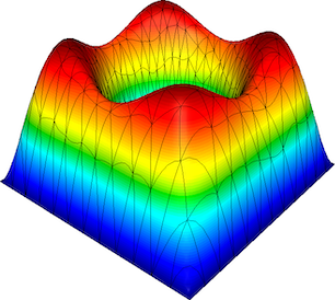
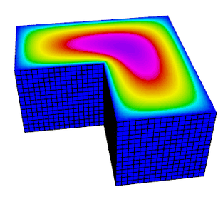
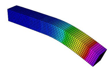
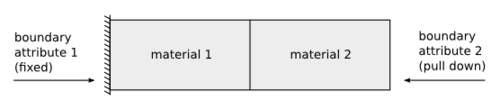
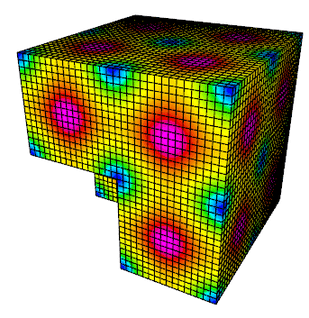
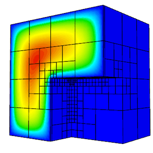
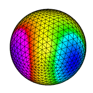
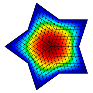
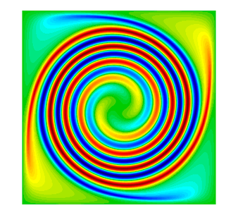
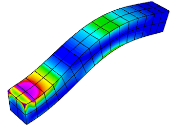
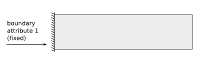
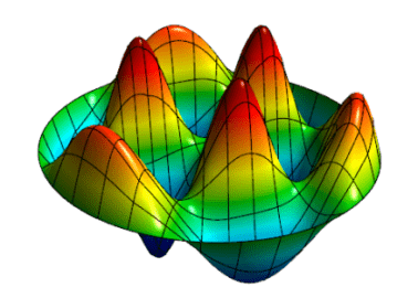
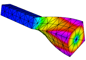
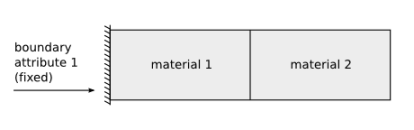
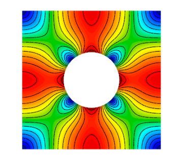
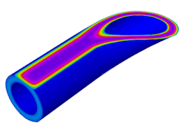
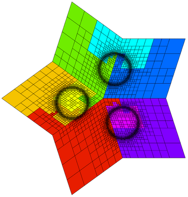
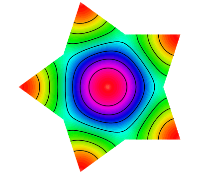
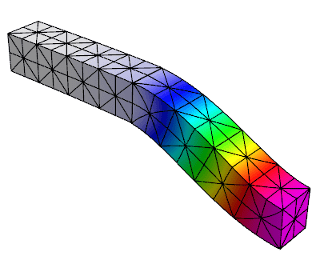
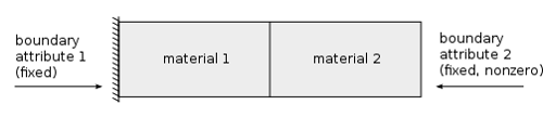
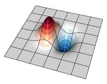
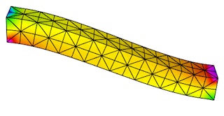
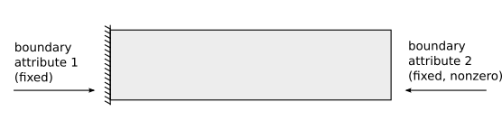

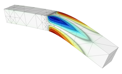
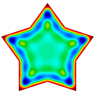
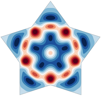
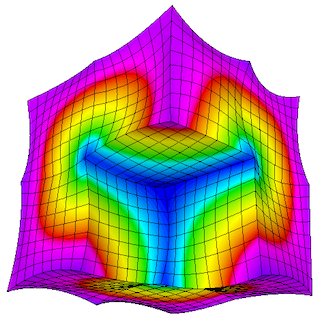

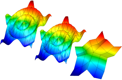
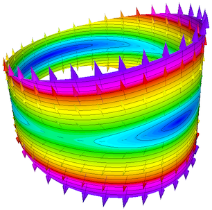
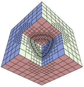
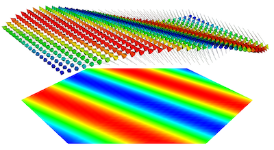
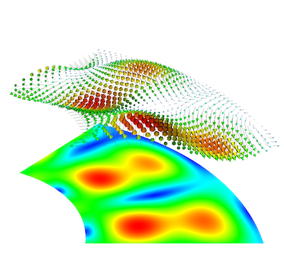
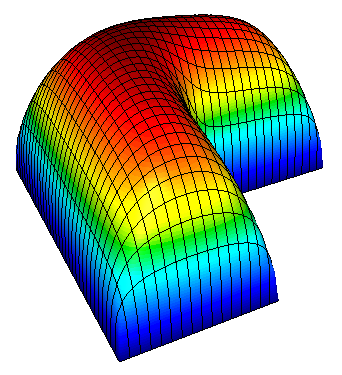
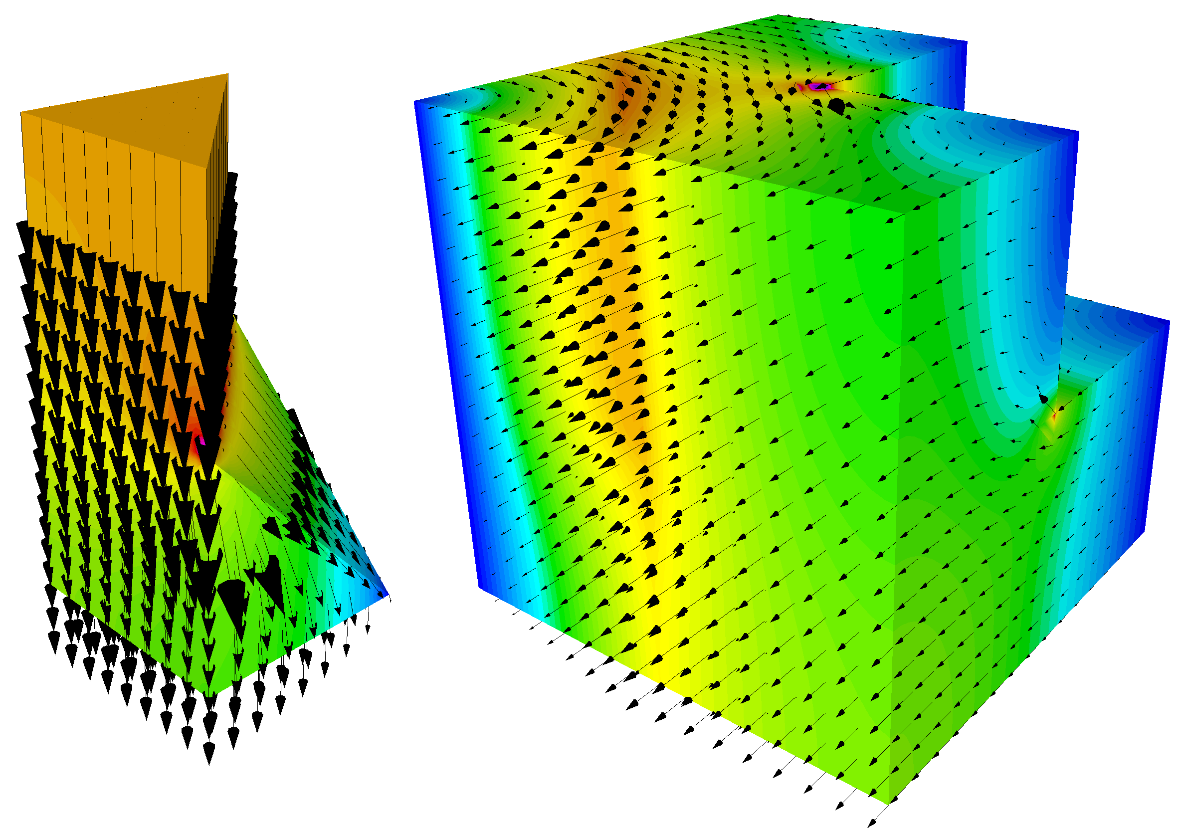
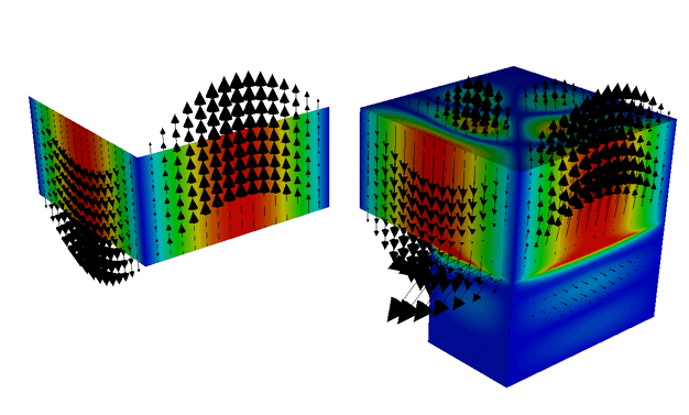
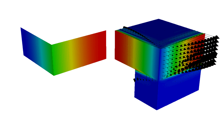 In Example 22 this boundary condition was simply a constant in space. In this
example the boundary condition is an eigenmode of a lower dimensional
eigenvalue problem defined on a portion of the boundary as follows:
In Example 22 this boundary condition was simply a constant in space. In this
example the boundary condition is an eigenmode of a lower dimensional
eigenvalue problem defined on a portion of the boundary as follows:


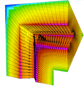
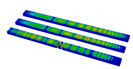
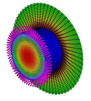
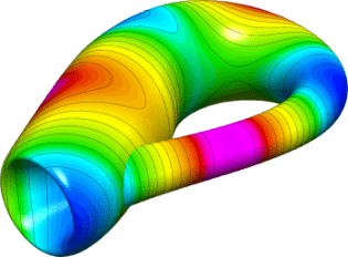


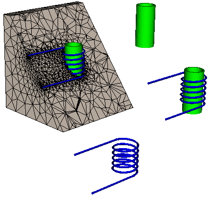


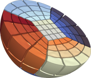

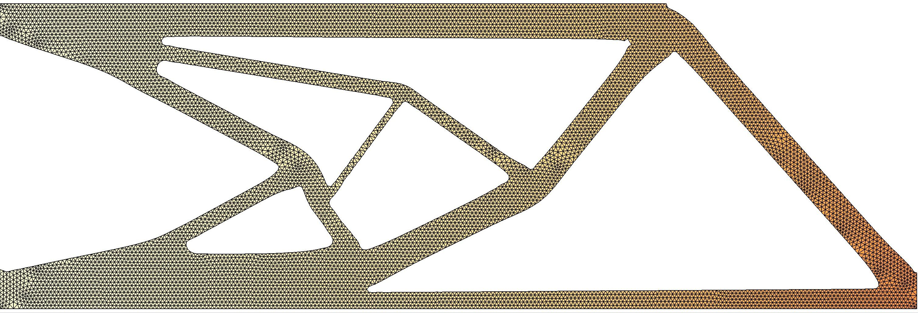

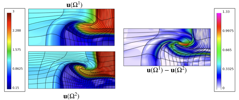
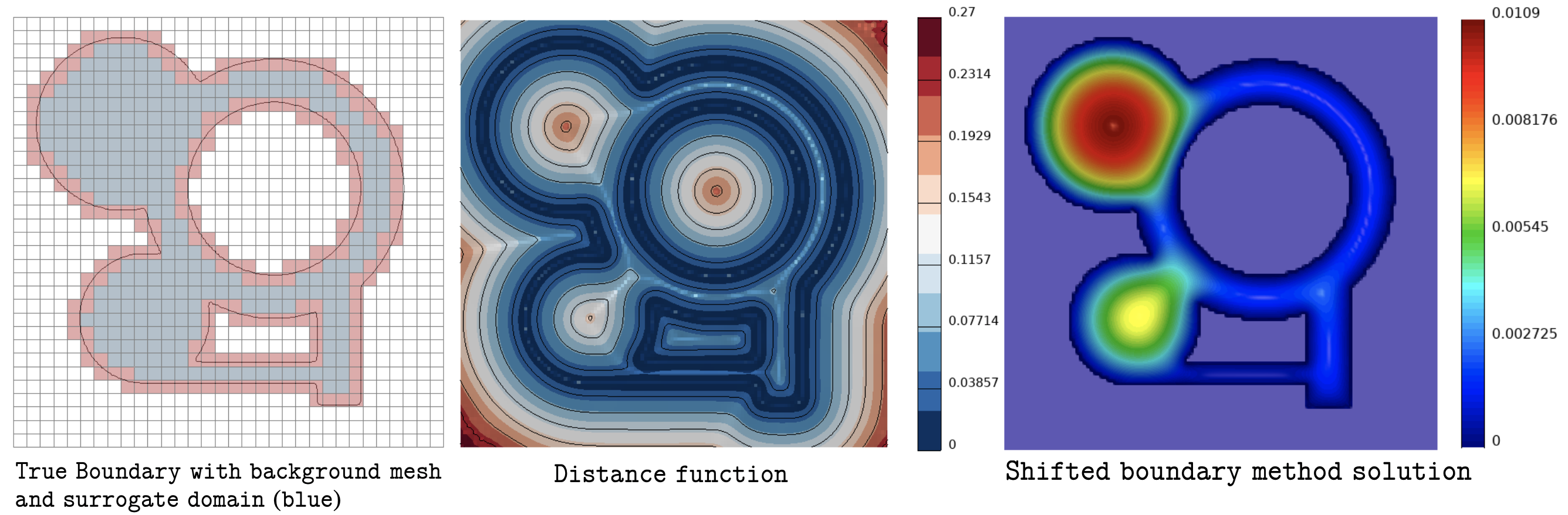

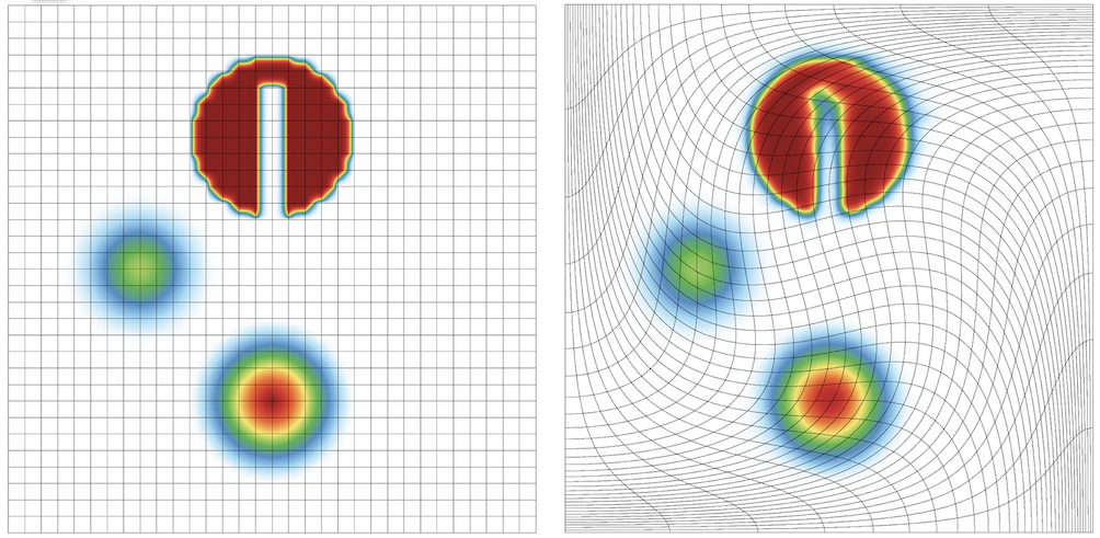
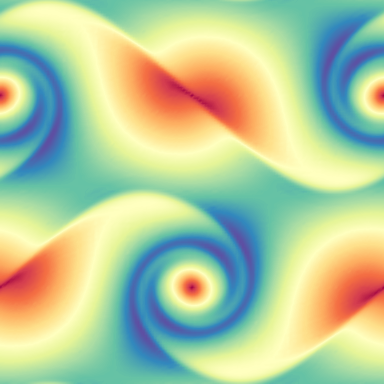
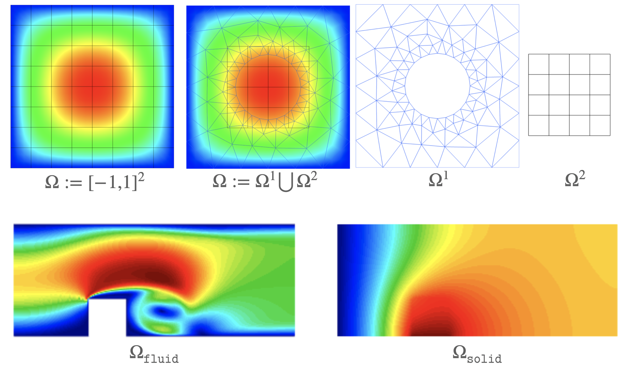
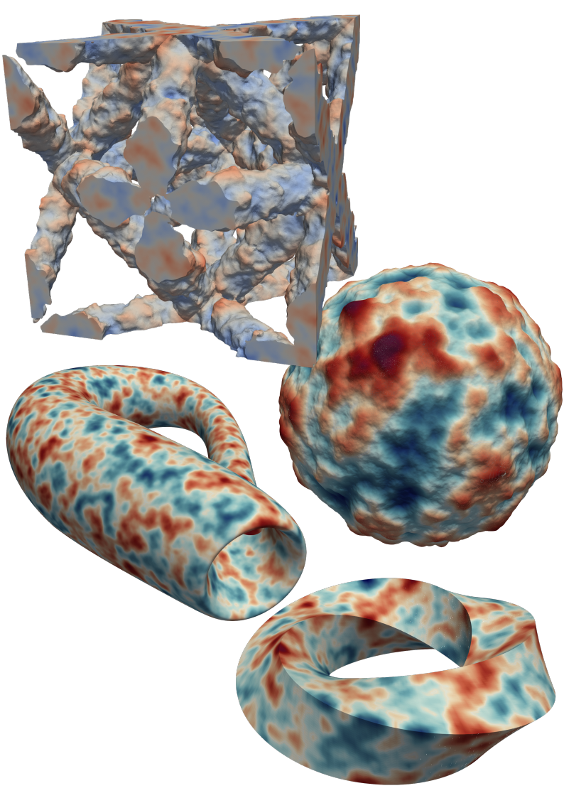
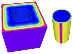
 This example solves the simple Poisson equation $$-Δ u = f$$ and computes rates of convergence under successive uniform h-refinements for a smooth manufactured solution. The parallel version also includes an AMR implementation for the L-shape benchmark problem. This example has a serial (
 This example solves the
convection-diffusion problem:
\begin{align}
-\epsilon \Delta u + \nabla \cdot (\beta u) &= f\\
\end{align}
using AMR. The example demonstrates the use of mesh-dependent test norms which are suitable for problems with solutions that exhibit large gradients present in internal or boundary layers. The example has a serial (
This example solves the
convection-diffusion problem:
\begin{align}
-\epsilon \Delta u + \nabla \cdot (\beta u) &= f\\
\end{align}
using AMR. The example demonstrates the use of mesh-dependent test norms which are suitable for problems with solutions that exhibit large gradients present in internal or boundary layers. The example has a serial ( This example solves the indefinite Helmholtz equation
\begin{align}
-\Delta u - \omega^2 u &= f\\
\end{align}
The example includes formulations with manufactured plane-wave solutions as well as high-frequency scattering problems and the use of Perfectly Match Layers (PML). It also demonstrates how to set up complex-valued systems and preconditioners for their solutions.
The example has a serial
(
This example solves the indefinite Helmholtz equation
\begin{align}
-\Delta u - \omega^2 u &= f\\
\end{align}
The example includes formulations with manufactured plane-wave solutions as well as high-frequency scattering problems and the use of Perfectly Match Layers (PML). It also demonstrates how to set up complex-valued systems and preconditioners for their solutions.
The example has a serial
( This example solves
the indefinite Maxwell problem
\begin{align}
\nabla × (\mu^{-1} \nabla \times E) - \omega^2 \epsilon E&= J\\
\end{align}
The example includes formulations with smooth manufactured solutions, AMR formulations for high-frequency scattering problems as well as a problem with a singular solution. The example has a serial
(
This example solves
the indefinite Maxwell problem
\begin{align}
\nabla × (\mu^{-1} \nabla \times E) - \omega^2 \epsilon E&= J\\
\end{align}
The example includes formulations with smooth manufactured solutions, AMR formulations for high-frequency scattering problems as well as a problem with a singular solution. The example has a serial
(