Primal and Dual Vectors
The finite element method uses vectors of data in a variety of ways and the
differences can be subtle. MFEM defines GridFunction, LinearForm, and
Vector classes which help to distinguish the different roles that vectors of
data can play.
Primal Vectors
The finite element method is based on the notion that a smooth function can be approximated by a sum of piece-wise smooth functions (typically piece-wise polynomials) called basis functions: $$f(\vec{x})\approx\sum_i f_i \phi_i(\vec{x}) \label{expan}$$ The support of an individual basis function, $\;\phi_i(\vec{x})$, will either be a single zone or a collection of zones that share a common vertex, edge, or face. The expansion coefficients, $\;f_i$, are linear functionals of the field being approximated, $\;f(\vec{x})$ in this case. The $\;f_i$ could be as simple as values of the function at particular points, called interpolation points, e.g. $\;f_i=f(\vec{x}_i)$, or they could be integrals of the field over submanifolds of the domain, e.g. $\;f_i = \int_{\Omega_i}f(\vec{x})d\vec{x}$. There are many possibilities but the expansion coefficients must be linear functionals of $\;f(\vec{x})$. The expansion coefficients are often called degrees of freedom, or DoFs for short, though in certain cases they may not be actually independent because of some problem specific constraints. We'll discuss this more in a later section on True DoFs.
Once the basis functions are defined, with some unique ordering, the expansion
coefficients can be stored in a vector using the same order. Such a vector of
coefficients is called a primal vector. The original function,
$\;f(\vec{x})$, can then be approximated using \eqref{expan}. In practice this
requires not only the primal vector of coefficients but also knowledge of the
mesh and the basis functions for each element of the mesh. In MFEM these
collections of information are combined into GridFunction objects (or
ParGridFunction objects when used in parallel) which represent piece-wise
functions belonging to a finite element approximation space.
The GridFunction class contains many Get methods which can compute the
expansion \eqref{expan} at particular locations within an element. The primal
vector of expansion coefficients can be computed by solving a linear system or
by using any of the various Project methods provided by the GridFunction
class. These methods compute the degrees of freedom, $\;f_i$, or some subset
of them, from a Coefficient object representing $\;f(\vec{x})$.
Other methods in this class can be used to compute various measures of the
error in the finite element approximation of $\;f(\vec{x})$.
Dual Vectors
Any vector space, such as the space of primal vectors, has a dual space containing co-vectors a.k.a. dual vectors. In this context a dual vector is a linear functional of a primal vector meaning that the action of a dual vector upon a primal vector is a real number. For example, the integral of a field over a domain, $\;\alpha=\int_\Omega g(\vec{x})d\vec{x}$, is a linear functional because the integral is linear with respect to the function being integrated and the result is a real number. Indeed we can derive similar linear functionals using compatible functions, $\;f(\vec{x})$, in a variety of ways, for example $G(f)=\int_\Omega g(\vec{x})f(\vec{x})d\vec{x}$. If we compute the action of our functional on the finite element basis functions, $$G_i=G(\phi_i(\vec{x})) = \int_\Omega g(\vec{x})\phi_i(\vec{x})d\vec{x}\label{dualvec},$$ and we collect the results into a vector with entries $\;G_i$, we call this a dual vector of $\;g(\vec{x})$.
Integrals such as this often arise when enforcing energy balance in physical systems. For example, if $\vec{J}$ is a current density describing a flow of charged particles and $\vec{E}$ is an electric field acting upon those particles, then $\int_\Omega\vec{J}\cdot\vec{E}\,d\vec{x}$ is the rate at which work is being done by the field on the charged particles.
MFEM provides LinearForm objects (or ParLinearForm objects in parallel)
which can compute dual vectors from a given function, $\;g(\vec{x})$,
described by a Coefficient object.
(Par)LinearForm objects require not only the mesh, basis functions, and the
field $\;g(\vec{x})$ but also a LinearFormIntegrator which defines precisely
what type of linear functional is being computed.
See Linear Form Integrators for more information about MFEM's
linear form integrators.
If, instead of a Coefficient object,
you have a primal vector, $\;g_j$, representing $\;g(\vec{x})$ you can form a
dual vector by multiplying $\;g_j$ by a bilinear form,
see Bilinear Form Integrators for more information on
bilinear forms. To understand why this is so, consider inserting the expansion
\eqref{expan} into \eqref{dualvec}.
$$
G_i=\int_\Omega \left(\sum_j g_j \phi_j(\vec{x})\right)\phi_i(\vec{x})d\vec{x}
= \sum_j \left(\int_\Omega \phi_j(\vec{x})\phi_i(\vec{x})d\vec{x}\right)g_j
\label{dualvecprod}$$
The last integral contains two indices and can therefore be viewed as an entry
in a square matrix. Furthermore, each dual vector entry, $\;G_i$, is
equivalent to one row of a matrix-vector product between this matrix of basis
function integrals and the primal vector $\;g_j$. This particular matrix,
involving only the product of basis functions, is traditionally called a
mass matrix. However, the action of any matrix, resulting from a bilinear
form, upon a primal vector will produce a dual vector. In general, such
dual vectors will have more complicated definitions than \eqref{dualvec} or
\eqref{dualvecprod} but they will still be linear functionals of primal
vectors.
True Degree-of-Freedom Vectors
Primal vectors contain all of the expansion coefficients needed to compute the finite element approximation of a function in each element of a mesh. When run in parallel, the local portion of a primal vector only contains data for the locally owned elements. Regardless of whether or not the simulation is being run in parallel, some of these coefficients may in fact be redundant or interdependent.
Sources of redundancy:
- In parallel some coefficients must be shared between processors.
- When using static condensation or hybridization many coefficients will depend upon the coefficients which are associated with the skeleton of the mesh as well as upon other data.
- When using non-conforming meshes some of the coefficients on the finer side of a non-conforming interface between elements will depend upon those on the coarser side of the interface.
For any or all of these reasons primal vectors may not contain the true degrees-of-freedom for describing a finite element approximation of a field. The true set of degrees-of-freedom may in fact be much smaller than the size of the primal vector.
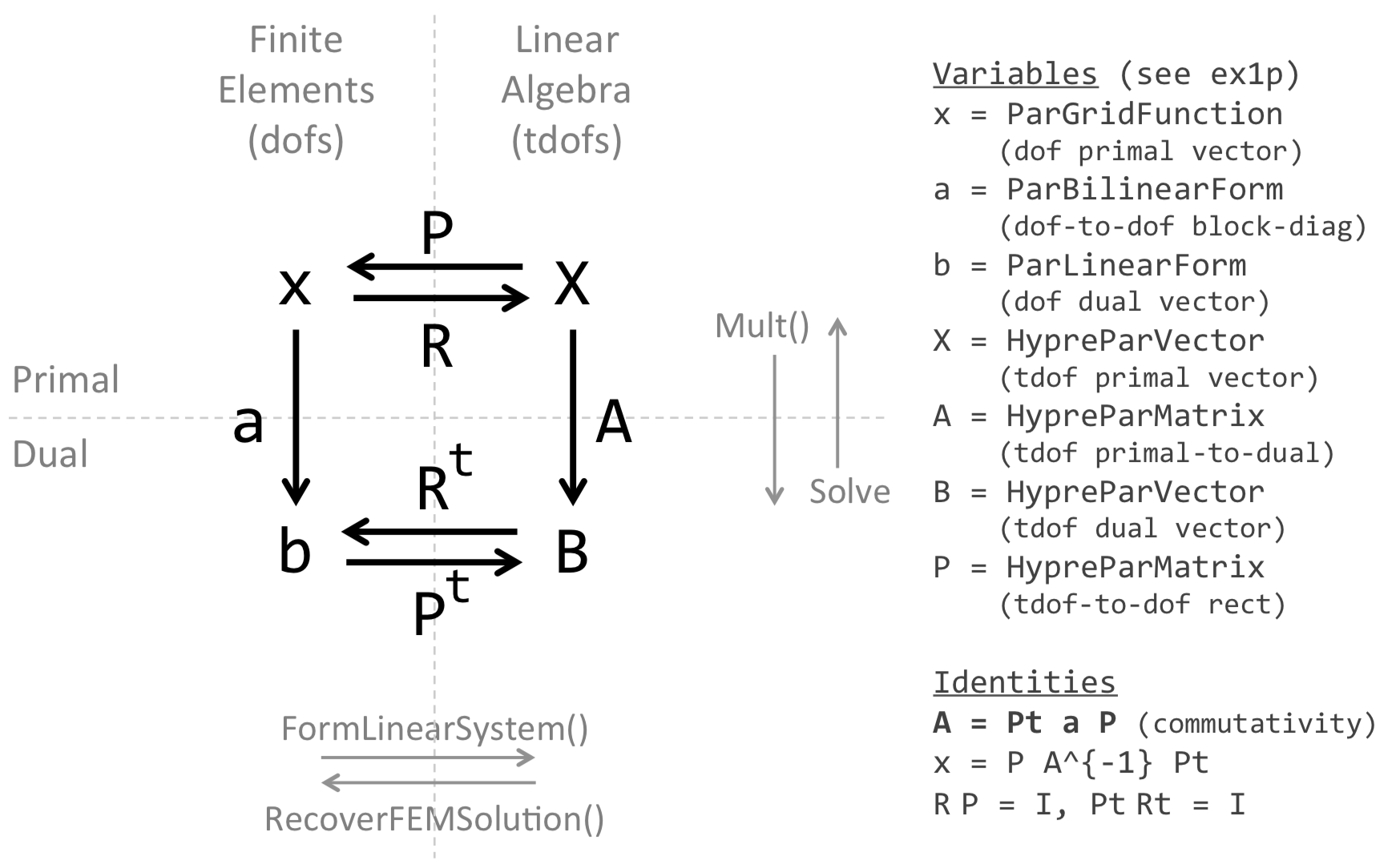
When setting up and solving a linear system to determine the finite element
approximation of a field, the size of the linear system is determined by the
number of true degrees-of-freedom. The details of creating this linear
system are mostly hidden within the BilinearForm object. To convert
individual bilinear form objects the user can call the
BilinearForm::FormSystemMatrix() method, however, the more common task is to
form the entire linear system with BilinearForm::FormLinearSystem(). As
input, this method requires a primal vector, a dual vector, and an array of
Dirichlet boundary degree-of-freedom indices. The degree-of-freedom array
contains the true degrees-of-freedom, as obtained from a FiniteElementSpace
object, which coincide with the Dirichlet, a.k.a. essential, boundaries.
// Given a bilinear form 'a', a primal vector 'x', a dual vector 'b',
// and an array of essential boundary true dof indices...
SparseMatrix A;
Vector B, X;
a.FormLinearSystem(ess_tdof_list, x, b, A, X, B);

// Solve X = A^{-1}B
...

a.RecoverFEMSolution(X, b, x);
The primal vector
must contain the appropriate values for the solution on the essential
boundaries. The interior of the primal vector is ignored by default although
it can be used to supply an initial guess when using certain solvers. The dual
vector should be an assembled LinearForm object or the product of a
GridFunction and a BilinearForm. As output,
BilinearForm::FormLinearSystem() produces the objects $A$, $X$, and $B$ in
the linear system $A X=B$. Where $A$ is ready to be passed to the appropriate
MFEM solver, $X$ is properly initialized, and $B$ has been modified to
incorporate the essential boundary conditions. After the linear system has
been solved the primal vector representing the solution must be built from $X$
and the original dual vector by calling BilinearForm::RecoverFEMSolution().
Technical Details
Constructing Dual Vectors
It was mentioned above, in the section on
Dual Vectors, that you can create a dual vector
by multiplying a primal vector by a bilinear form. But of course if you have a
primal vector you can also use a GridFunctionCoefficient to create a dual
vector using a LinearForm and an appropriate LinearFormIntegrator. These
two choices should produce nearly identical results if the
BilinearFormIntegrator and the LinearFormIntegrator use the same
integration rule order. The order of the summation might differ between
BilinearFormIntegrator and LinearFormIntegrator, potentially resulting in
round-off error differences.
When considering to use a BilinearForm or a LinearForm, one must be aware of
their different computational and memory costs. A bilinear form must create a
sparse matrix which can require a great deal of memory. Integrating a
GridFunctionCoefficient in a LinearForm object will require very little
memory. On the other hand, computing the integrals inside a LinearForm
object can be computationally expensive even in comparison to assembling the
bilinear form.
Which is the better option? As always, there are trade-offs. The answer
depends on many variables; the complexities of the BilinearFormIntegrator and
the LinearFormIntegrator, the complexity of other coefficients that may be
present, the order of the basis functions, can the bilinear form be reused or
is this a one-time calculation, whether the code runs on a CPU or GPU, etc. On
some architectures the motion of data through memory during a matrix-vector
multiplication may be expensive enough that using a LinearForm and
recomputing the integrals is more efficient.
Often the construction of dual vectors is a small portion of the overall compute time so this choice may not be critical. The best choice is to test your application and determine which method is more appropriate for your algorithm on your hardware.