Basis Functions

The finite element method is based on the notion that a smooth function can be approximated by a linear combination of piece-wise smooth functions (typically piece-wise polynomials) called basis functions. The coefficients of the linear combination are called degrees of freedom (DoFs) and are linear functionals of the approximated function, e.g. values at interpolation points or integrals over sub-manifolds of the domain. No matter the space the problem is formulated in, H1, H(curl), H(div) or L2, or more precisely the discrete space the problem is weakly-formulated in, there is an infinite range of possible bases spanning the very same discrete space.

One-Dimensional Polynomial Bases

Consider the $[0,1]$ interval on the real line and the space of real, univariate polynomials of degree less than or equal to $n$. Any set ${l_{j \in {0,...,n}}}$ of $n+1$ linearly independent polynomials of degree less than or equal to $n$ forms a basis of this space. We say a basis interpolates a given node $x$ if, for one of the basis functions $l_{j'}$ we have $l_{j'}(x)=1$, and $l_{j \neq j'}(x)=0$. We distinguish between open and closed bases. An open basis does not interpolate the interval endpoints, whereas a closed basis does. If a basis is entirely interpolatory on a set of nodes $x_{i \in {0,...,n}}$ in the sense that $l_j(x_i)=\delta_{ij}$, i.e. is a Lagrange basis, we call it a nodal basis and all its associated DoFs correspond to values of the approximated function.

Cubic basis functions on [0,1]

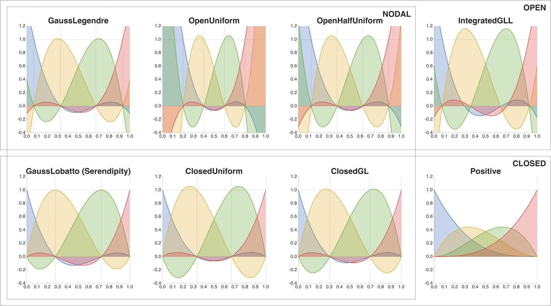
• GaussLegendre: open and nodal basis; the basis of order $n$ interpolates all the quadrature points of the Gauss-Legendre quadrature rule with $n+1$ points. These points are the zeros of the Legendre polynomial of degree $n+1$.

• OpenUniform: open and nodal basis; the basis of order $n$ interpolates all the quadrature points of an open Newton-Cotes quadrature rule with $n+1$ equidistant points. These points partition the $[0,1]$ interval in $n+2$ subintervals of equal length, $x_{i \in {0,...,n}} = (i+1)/(n+2)$.

• OpenHalfUniform: open and nodal basis; the basis of order $n$ interpolates all the quadrature points of an open Newton-Cotes quadrature rule with $n+1$ equidistant points. These are the midpoints of $n+1$ subintervals of equal length partitioning the $[0,1]$ interval, $x_{i \in {0,...,n}} = (1/2+i)/(n+1)$.

• IntegratedGLL: open basis; the basis of order $n$ histopolates all the subintervals in-between the quadrature points of the Gauss-Lobatto quadrature rule with $n+2$ points. These points are the $[0,1]$ interval endpoints plus the zeros of the first derivative of the Legendre polynomial of degree $n+1$. The integral of each basis function over its respective subinterval equals one (or, alternatively, the length of the subinterval) and is zero over all other $n$ subintervals, meaning that all DoFs associated with this basis correspond to integrals (or, alternatively, mean values) of the approximated function over the respective subinterval. See also Gerritsma, M. (2011). Edge Functions for Spectral Element Methods.

• GaussLobatto: closed and nodal basis; the basis of order $n$ interpolates all the quadrature points of the Gauss-Lobatto quadrature rule with $n+1$ points. These points are the $[0,1]$ interval endpoints plus the zeros of the first derivative of the Legendre polynomial of degree $n$.

• ClosedUniform: closed and nodal basis; the basis of order $n$ interpolates all the quadrature points of the closed Newton-Cotes quadrature rule with $n+1$ equidistant points. These points partition the $[0,1]$ interval in $n$ subintervals of equal length, $x_{i \in {0,...,n}} = i/n$.

• ClosedGL: closed and nodal basis; the basis of order $n$ interpolates the $[0,1]$ interval endpoints plus the midpoints of the subintervals in-between all the quadrature points of the Gauss-Legendre quadrature rule with $n$ points.

• Positive: closed basis; the basis of order $n$ is simply the Bernstein polynomial basis of degree $n$ and only interpolates the $[0,1]$ interval endpoints, $b_{i \in {0,...,n}}(x) = {n \choose i} x^{i}(1-x)^{n-i}$.

The Poly_1D::Basis class includes member functions capable of evaluating all of the aforementioned bases, as well as their first and second derivatives, at an arbitrary point in the $[0,1]$ interval. In addition, the enclosing Poly_1D class includes facilities to compute real, univariate polynomials forming hierarchical bases, including monomials, Chebyshev, and Legendre polynomials.

Finite Element Collections and Elements of Different Types

When constructing a finite element collection for a given order and dimension, the user can often specify one, for H1 and L2 spaces, or two, for ND and RT spaces, of the one-dimensional bases described above. In most cases the user can simply use the provided defaults, Gauss-Lobatto for H1 spaces, Gauss-Lobatto plus Gauss-Legendre for ND and RT spaces, and Gauss-Legendre for L2 spaces. This should not be confused with the integration rule default, which remains Gauss-Legendre for all cases.

For tensor product elements, e.g. quadrilaterals or hexahedra, the basis functions are just products of one-dimensional closed and/or open basis functions. Alternatively, for order two and above, the smaller serendipity basis, produces smaller system operators while converging at the same rate. Note that support for serendipity hexahedral elements is still work in progress and that for order one or in one dimension, the serendipity basis degenerates into the Gauss-Lobatto basis described above. For simplices, e.g. triangles or tetrahedra, the process of constructing the basis functions is slightly more involved, but can essentially be pictured as starting from the one-dimensional bases above and extending in a triangular lattice on the faces and in the interior, thus retaining their property as open, closed and/or nodal. In practice, in MFEM, the basis functions for simplices are obtained as products of a hierarchical, one-dimensional basis of Chebyshev polynomials of the first kind. Triangular prisms and, more generally, wedge elements are the tensor product of a triangle and segment element, while pyramids are based on Fuentes, F. et al. (2015). Orientation embedded high order shape functions for the exact sequence elements of all shapes.

The user can use the display-basis miniapp to visualize various types of basis functions on a single mesh element of their choice.

Some Notes on Choosing Basis Functions

Occasionally, the user might find the default basis functions are not suitable for a given problem formulation. The following is a non-exhaustive list of considerations to take into account when choosing what basis functions to use.

First, due to their nature, not all collections accept all function bases. For instance, H1 spaces are continuous and thus require a basis which is interpolatory at the element boundaries, i.e. a closed basis. On the contrary, L2 spaces do not necessarily have DoFs at the element boundaries and can be spanned by an open basis, or any basis in fact. If an open basis is selected though, extra care is needed in order to specify Dirichlet boundary conditions.

Next, nodal basis functions are particularly simple and efficient to evaluate due to barycentric interpolation, and to integrate, especially if the user were to write their own assembly routines using the corresponding collocated quadrature rule.

Finally, Low-Order-Refined (LOR) discretizations are only spectrally equivalent to the original high-order system if using a Gauss-Lobatto basis for H1 spaces and Gauss-Lobatto plus IntegratedGLL bases for both ND and RT spaces. Note that if a different choice is made, MFEM issues a warning but will still proceed.